3712
Super resolution imaging from low-field strength scanners using generative adversarial networks1Bioengineering, University of Pennsylvania, Philadelphia, PA, United States, 2National Institute of Neurological Disorders and Stroke, Bethesda, MD, United States, 3Biostatistics, University of Pennsylvania, Philadelphia, PA, United States, 4Hyperfine, Guilford, CT, United States, 5Radiology, University of Pennsylvania, Philadelphia, PA, United States, 6Neurology, University of Pennsylvania, Philadelphia, PA, United States
Synopsis
Keywords: Machine Learning/Artificial Intelligence, Low-Field MRI, super resolution
High-field MRI provides superior imaging for diverse clinical applications, but cost and other factors limit availability in various healthcare and lower resource settings. Lower-field strength units promise to expand access but involve tradeoffs including reduced signal, longer scan times, and lower resolution. Here we develop super-resolution methods that can generate high-field quality images from low-field scanner inputs, thus increasing signal and resolution. We use generative adversarial networks to demonstrate image enhancement in T1, T2 and FLAIR sequences.Introduction
Recently, there has been renewed academic and commercial interest in lower-field strength scanners.1 While low-field scanners have shown promise in a variety of clinical applications,2–4 obtaining diagnostic quality sequences on these lower magnetic field strength devices requires careful balancing of scan parameters.5 In order to maintain clinically relevant acquisition times, low-field sequences often have reduced signal and lower resolution. Generative adversarial networks (GANs) have emerged as a powerful deep-learning-based technique that have been applied to a variety of image enhancement problems.6 Here, we apply GANs to a dataset of same-day, paired high-field and low-field imaging to enhance the image quality of low-field images.Methods
2.1 DatasetTo develop the super-resolution algorithms, we used a dataset of 36 head MRIs obtained from patients with multiple sclerosis at two academic hospitals. Each patient underwent whole-brain imaging on 3T scanners (Siemens, Erlangen, Germany) with 3D T1-weighted (T1w), T2-weighted (T2w), and 3D T2-FLAIR sequences, though sequence parameters varied between sites. Each patient underwent same-day whole-brain low-field imaging using a 64mT portable scanner (Hyperfine, Guilford, CT) with 3D fast spin-echo T1w, T2w, and T2-FLAIR scans in the axial plane. Low-field protocols were identical between sites. Each patient in the dataset was subsequently randomized to a training (N=24), validation (N=6), or test (N=6) set for machine learning model development.
2.2 Preprocessing
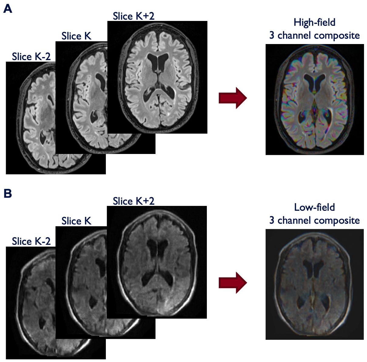
All scans were first resliced to 1mm isotropic resolution. Paired high-field imaging was then coregistered to low-field imaging using a dense rigid registration with Advanced Normalization Tools (ANTs). Each 3D acquisition was normalized to a 0 to 255 range, padded to square in the axial plane, and output as a series of jpg files. To encode some 3D information into the 2D jpg files, we incorporated adjacent slices into the 3 RGB channels of each jpg file (Figure 1). This 2.5D approach permits the model to access information about neighboring slices which can result in reduced image artifacts and improved continuity between slices. For each sagittal slice (K) in the dataset, the additional 2 RGB channels were filled with values from K+2 and K-2 slices (i.e. 2 mm distance from the central slice).
2.3 Model training
To enhance the low-field images, we employed the pix2pix paired Generative Adversarial Network (GAN) with PyTorch backend (https://github.com/junyanz/pytorch-CycleGAN-and-pix2pix).7 This model consists of a generator (Unet-256) and a discriminator (70x70 patchGAN). Models were trained for 100 epochs using a learning rate of 2e-4 with linear decay after 30 epochs and a batch size of 32. Training data were augmented using random horizontal flipping.
2.4 Model evaluation and statistics
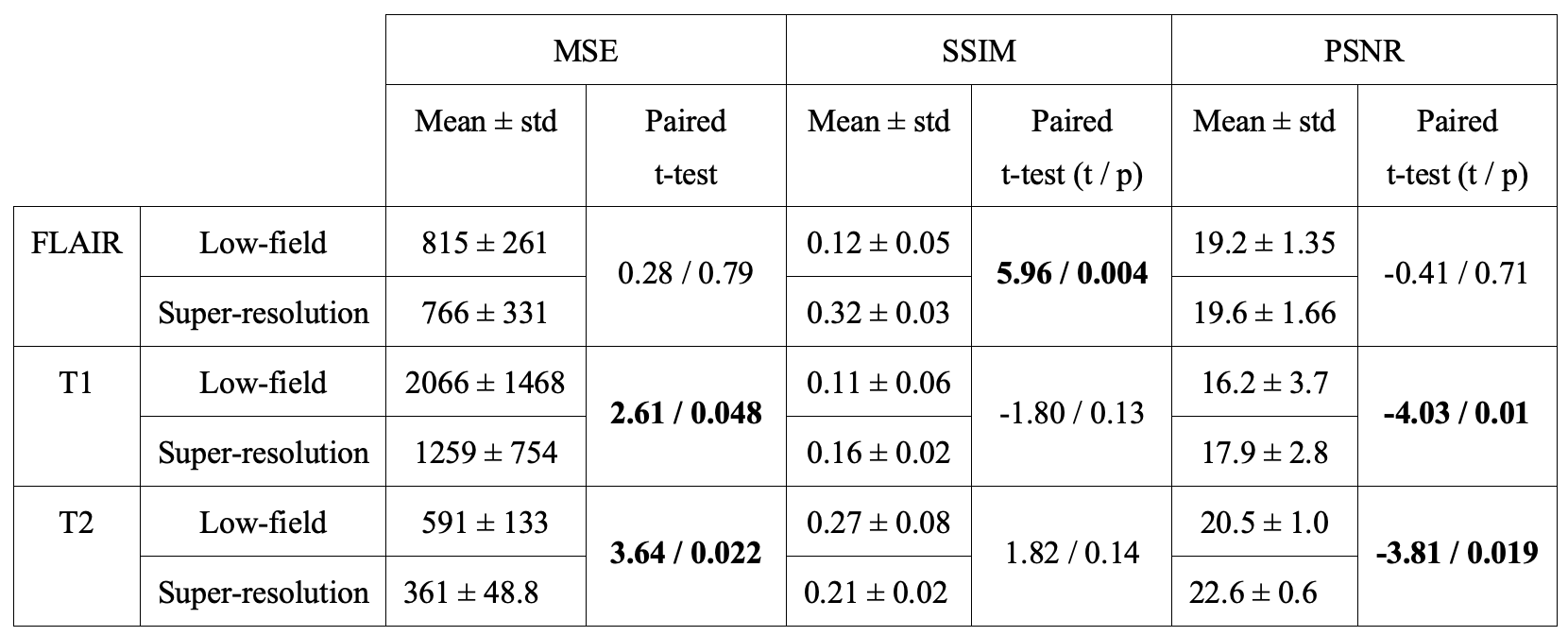
Model performance was assessed on the held-out test set (N=6) using three quantitative metrics: mean squared error (MSE), structural similarity index measure (SSIM), and peak signal-to-noise ratio (PSNR). For each quantitative metric, we used subject-level paired t-tests to compare the low-field and super-resolution enhanced imaging. All statistics were generated using scipy (v1.7.3), numpy (v1.21.6), and seaborn (v0.12.1) in Python (v3.7.5).
Results
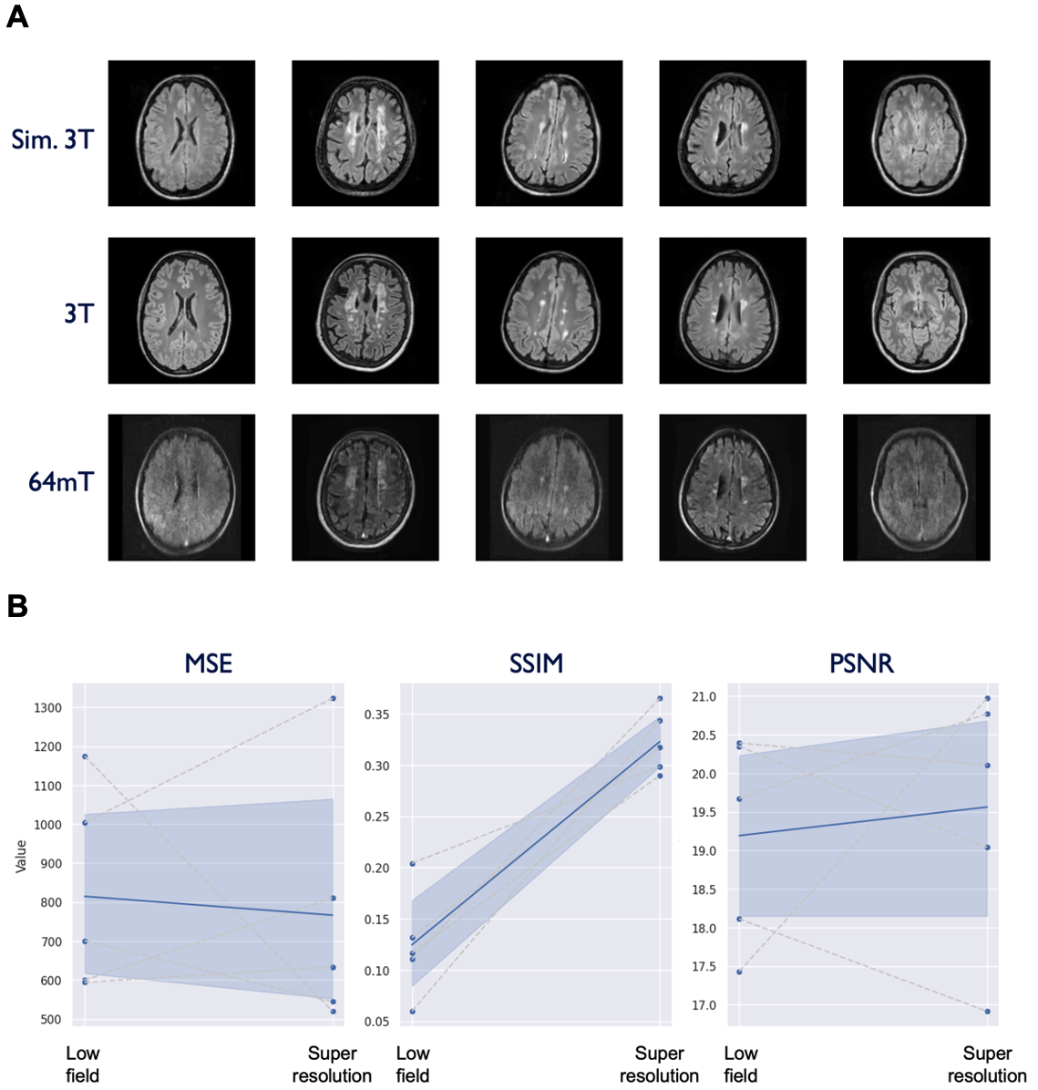
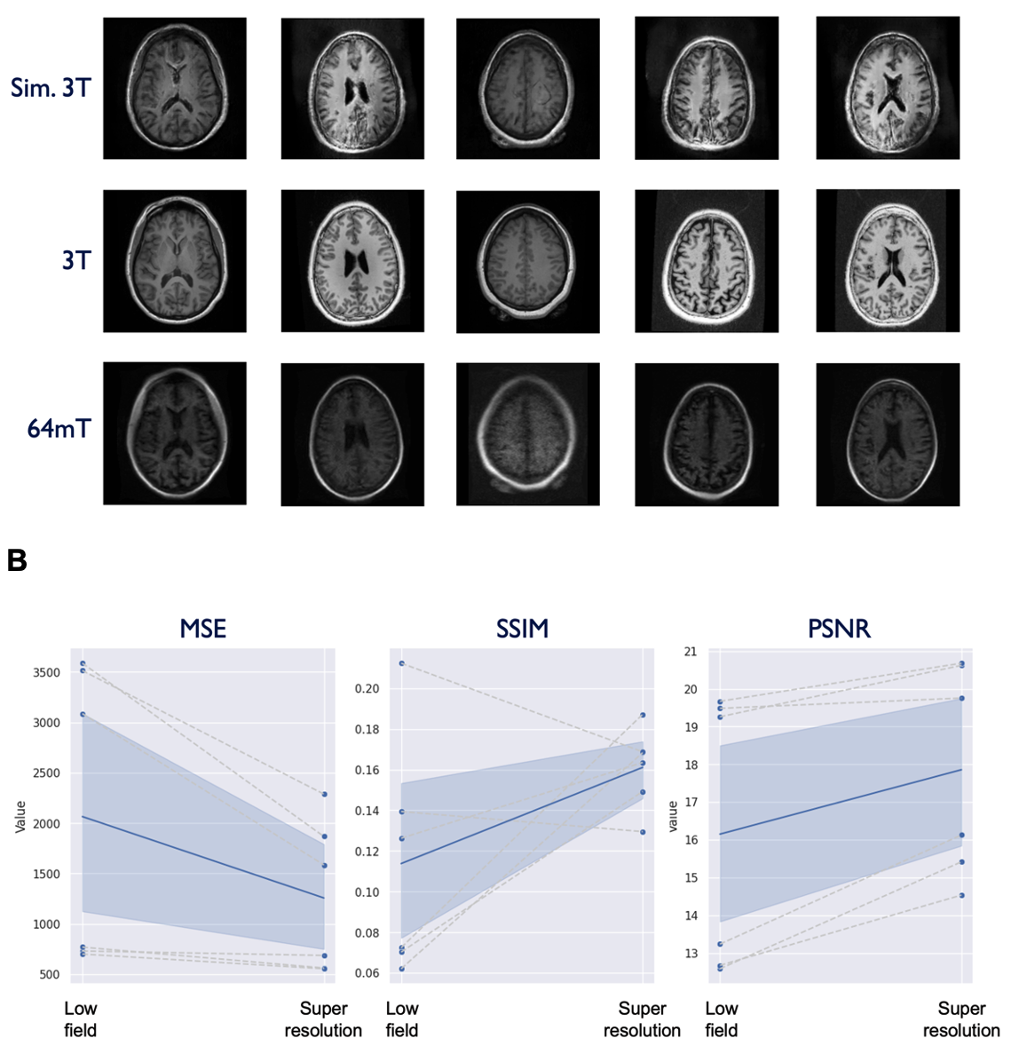
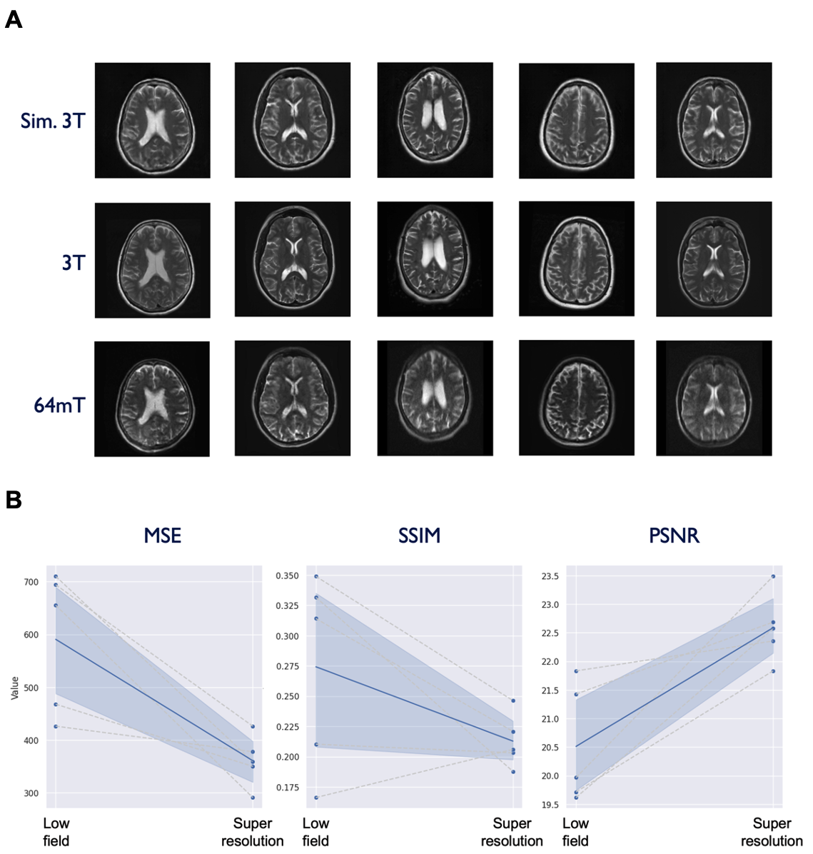
Model performance was assessed on the test set (N=6) using the three quantitative metrics: MSE, SSIM, and PSNR. For reference, we also applied these quantitative metrics to the non-enhanced low-field data. The models for T1 and T2 enhancement showed a significant improvement in MSE (T1: p = 0.048, T2: p = 0.022) and PSNR (T1: p = 0.01, T2: p = 0.019), though no effect was found for SSIM. The FLAIR model demonstrated SSIM improvement (p = 0.004), but no effect was seen for MSE and PSNR. Table 1 lists summary statistics and statistical comparisons for each metric. Figures 2-4 illustrate model performance for FLAIR, T1, and T2 sequences respectively.Discussion
In this project, we developed a GAN that takes low-field scans as input and attempts to generate high-field quality images as output. While this initial effort demonstrates promise in a limited context, there are a number of limitations to the model as it has been developed and there are significant opportunities for further model improvement. First, we utilized a limited dataset containing only axial head images. While our approach was sufficient within this limited dataset, it is unlikely to generalize to new scanners and anatomical structures. More aggressive data augmentation techniques could be one potential route to increase the robustness of the model. Additionally, there was some degree of discontinuity in pixel intensities between adjacent slices. While we employed a 2.5D approach to mitigate image artifacts and slice-to-slice discontinuity, it was limited to only 3 channels. In future work, additional slices and sequences could be encoded in additional channels. More advanced registration methods may also decrease differences between high-field and low-field datasets. Finally, augmenting the loss function to incorporate quantitative metrics may provide more relevant feedback to the model and further improve the perceived quality of the simulated images.Acknowledgements
Acknowledgements
We thank current and former team members at Hyperfine, Inc. (Guilford, CT), particularly Jonathan Rothberg, PhD, Samantha By, PhD, and Edward B. Welch, PhD, for technical assistance and the use of Hyperfine low-field MRI scanners. We thank the Penn Neuroradiology Research Core, including Brian Dolan, Marisa Sanchez, Leeanne Lezotte, Danielle Urban, and Lauren Karpf, for assistance with patient recruitment and scanning. We also acknowledge the staff of the NINDS Neuroimmunology Clinic; Rose Cuento, CRNP; and the staff of the NIH NMR Center.
Funding
T. Campbell Arnold was funded in part by the HHMI-NIBIB Interfaces Initiative (5T32EB009384-10). Additional support was provided by NINDS (DP1-NS122038, R56-NS099348, T32-NS091006) (BL), the Pennsylvania Health Research Formula Fund (BL), the Mirowski Family Fund (BL), the Jonathan Rothberg Family Fund (BL), and Neil and Barbara Smit (BL). This study received support from a research services agreement between Hyperfine, Inc. and the Trustees of the University of Pennsylvania (JMS). The study was partially funded by the Intramural Research Program of NINDS/NIH (DSR).
Disclosures
Sehat Okar, Karan Kawatra, and Govind Nair are supported by the Intramural Research Program of NINDS. John Pitts and Megan Poorman are employees of Hyperfine. Brian Litt is a co-founder of Liminal Science and serves on the Medical and Scientific Advisory Boards or Hyperfine and as a result has equity in the company. Russell T. Shinohara receives consulting income from Octave Bioscience, compensation for reviewing scientific articles from the American Medical Association and for reviewing grants for the Emerson Collective, National Institutes of Health, and the Department of Defense. Daniel S. Reich is supported by the Intramural Research Program of NINDS and additional research support from Abata and Sanofi-Genzyme. Joel M. Stein has received support from sponsored research agreements with Hyperfine and consulting income from Centaur Diagnostics, Inc.
References
1. Arnold TC, Freeman CW, Litt B, Stein JM. Low‐field MRI: Clinical promise and challenges. J Magn Reson Imaging. Published online September 19, 2022. doi:10.1002/jmri.28408
2. Sheth KN, Mazurek MH, Yuen MM, et al. Assessment of Brain Injury Using Portable, Low-Field Magnetic Resonance Imaging at the Bedside of Critically Ill Patients. JAMA Neurol. Published online September 8, 2020. doi:10.1001/jamaneurol.2020.3263
3. Arnold TC, Tu D, Okar S V., et al. Sensitivity of portable low-field magnetic resonance imaging for multiple sclerosis lesions. NeuroImage Clin. 2022;35:103101. doi:10.1016/j.nicl.2022.103101
4. Deoni SCL, Bruchhage MMK, Beauchemin J, et al. Accessible pediatric neuroimaging using a low field strength MRI scanner. Neuroimage. 2021;238:118273. doi:10.1016/j.neuroimage.2021.118273
5. Marques JP, Simonis FFJ, Webb AG. Low‐field MRI: An MR physics perspective. J Magn Reson Imaging. 2019;49(6):1528-1542. doi:10.1002/jmri.26637
6. Yi X, Walia E, Babyn P. Generative adversarial network in medical imaging: A review. Med Image Anal. 2019;58:101552. doi:10.1016/J.MEDIA.2019.101552
7. Zhu J-Y, Park T, Isola P, Efros AA, Research BA. Unpaired Image-to-Image Translation Using Cycle-Consistent Adversarial Networks Monet Photos.; 2017. Accessed November 9, 2022. https://github.com/junyanz/CycleGAN.
Figures