3701
Comparison of data-driven and physics-informed learning approaches for optimising multi-contrast MRI acquisition protocols1CUBRIC, Cardiff University, Cardiff, United Kingdom, 2Imaging Processing Laboratory, Universidad de Valladolid, Valladolid, Spain, 3SCIL, Université de Sherbrooke, Sherbrooke, QC, Canada, 4Centre for Medical Engineering, Centre for the Developing Brain, King's College London, London, United Kingdom, 5Image Sciences Institute, University Medical Centre Utrecht, Utrecht University, Utrecht, Netherlands
Synopsis
Keywords: Machine Learning/Artificial Intelligence, Data Acquisition, Quantitative Imaging
Multi-contrast MRI is used to assess the biological properties of tissues, but excessively long times are required to acquire high-quality datasets. To reduce acquisition time, physics-informed Machine Learning approaches were developed to select the optimal subset of measurements, decreasing the number of volumes by approximately 63%, and predict the MRI signal and quantitative maps. These selection methods were compared to a full data-driven and two manual strategies. Synthetic and real 5D-Diffusion-T1-T2* data from five healthy participants were used. Feature selection via a combination of Machine Learning and physics modelling provides accurate estimation of quantitative parameters and prediction of MRI signal.Introduction
Multi-contrast MRI experiments based on the variation of multiple acquisition parameters enables simultaneously assessment of different phenomena such as diffusion, relaxation, and susceptibility, and the extraction of joint and complementary information1. However, the high dimensionality of the acquisition parameter space can result in anexcessive number of measurements, prompting the development of biophysical modelling-based approaches to design efficient protocols2-5. Additionally, data-driven approaches can identify the best feature-subset selection to exploit the multi-contrast information6,7. In this work, we present combined machine learning and physics-informed approaches to select the optimal subset of measurements.Methods
DataFive healthy controls (labelled 1-5) were scanned on a 3T 40mT/m scanner with a 5D Diffusion-T1-T2* protocol varying b-value (b), gradient direction (Θg,Φg), inversion time TI and delay time TD using asymmetric spin echo6,8 (1344 unique settings). The data were preprocessed as previously described6.
Selection of optimal measurements
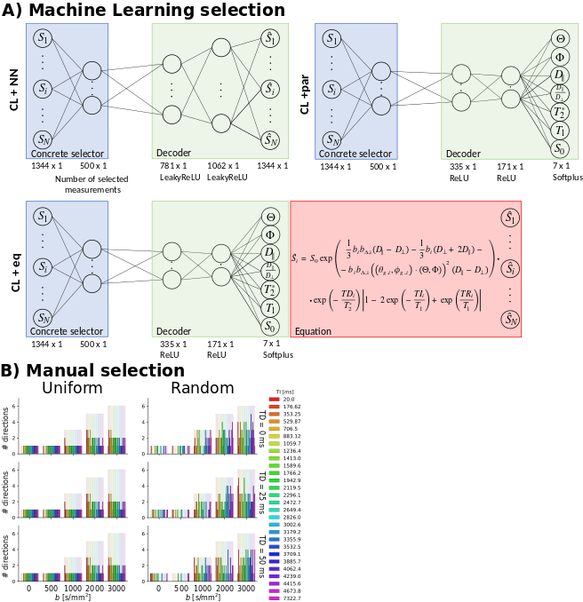
The extraction of the optimal subset of 500 MRI volumes was carried out with a regularised concrete autoencoder9-12. This approach has shown to predict non-acquired signals from a subset of measurements with higher accuracy than other techniques6. Specifically, the encoder of the network for the selection was based on a concrete selection layer (CL) that obtains the optimal measurements through stochastic linear combinations of input features11. The decoder was based on 1) a full data-driven technique using a neural network (CL+NN), 2) a combination of a neural network with a physics representation following a signal equation (CL+eq), or 3) directly optimising quantitative measures from estimation on the full dataset (CL+par) (Figure 1A). Additionally, two manual selection procedures were implemented: 4) a uniform reduction of gradient directions (Uniform); 5) a random selection of volumes (Random) (Figure 1B). CL+eq was based on the following equation8:
$$S=S_{0}e^{-\textbf{b}:\textbf{D}}\left|1-2e^{-\frac{\text{TI}}{\text{T1}}}+e^{-\frac{\text{TR}}{\text{T1}}}\right|e^{-\frac{\text{TD}}{\text{T2}^{*}}},(1)$$
where $$$\textbf{b}:\textbf{D}$$$ is:
$$\textbf{b}:\textbf{D}=\left( \frac{1}{3}bb_{\Delta}[\textbf{D}_{\parallel}-\textbf{D}_{\perp}]-\frac{1}{3}b[\textbf{D}_{\perp}+2\textbf{D}_{\parallel}]-bb_{\Delta}[(\Theta_{g},\Phi_{g})\cdot(\Theta,\Phi)]^{2}[\textbf{D}_{\parallel}-\textbf{D}_{\perp}]\right).(2)$$
Repetition time TR and $$$b_{\Delta}$$$ were 7500ms and 1, and the ranges of parameters were as follows: S0 [0.5-5], longitudinal relaxation time T1 [100-5000ms], transverse relaxation time T2* [0.01-2000ms], parallel diffusivity $$$D_{\parallel}$$$ [0.01-3.2μm2/ms], perpendicular diffusivity $$$D_{\perp}$$$ [k times $$$D_{\parallel}$$$, k=0.01-1], and first eigenvector angles Θ [0-π] and Φ [0-(2π-0.001)].
Experiments
All models were trained on real and synthetic data except CL+par, only trained on synthetic data. The synthetic volumes were obtained by fitting Eq. (1) to the full data using a neural network (CL+eq without the CL), and forward generating MRI signals to which Gaussian noise was added (signal-to-noise ratio SNR=30 for b=0, minimum TD and maximum TI volume).
Given the subset of selected measurements from each approach (1-5), parameter maps were estimated using a neural network equivalent to CL+eq without the CL, with the input size adjusted. The MRI signal was obtained following Eqs. (1-2).
Selection and estimation networks were trained based on leave-one-out cross-validation over all subjects using the Adam optimiser13 with learning rate 0.001, batch size 256, and mean-squared error (MSE) loss.
For synthetic data, the error of the quantitative measures was computed as the difference between the ground truth and estimated maps. For the first eigenvector, the error was computed from the dot product of the estimated and ground truth directions.
Results
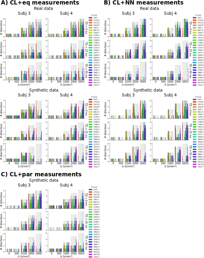
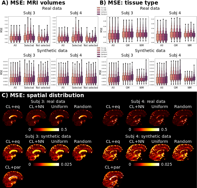
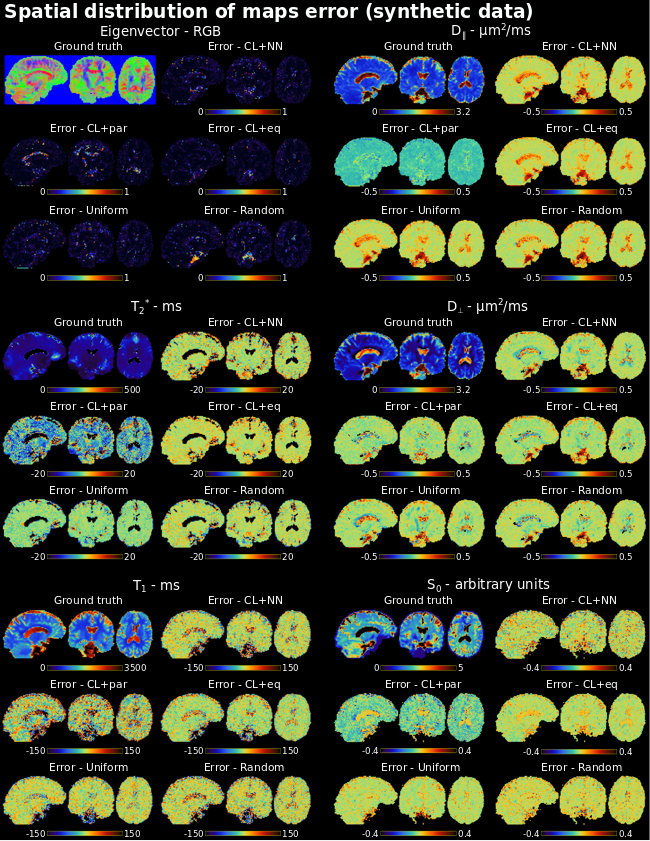
Regarding the selected measurements for the machine learning procedures, with CL+eq, a higher number of low SNR volumes (lowest TI together with high b-value) was selected (Figure 2).The MSE values of the predicted MRI signal were similar for all approaches except CL+par, which presented higher MSE (Figure 3).
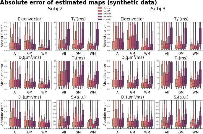
CL+eq showed a consistently lower error for the first eigenvector and T1 parameters than all other approaches, and, compared to CL+NN, lower values for the first eigenvector, $$$D_{\parallel}$$$, T2* and S0 (Figures 4-5). CL+par showed the highest error and bias for each parameter except the first eigenvector and $$$D_{\perp}$$$, with lower or similar error for the cerebrospinal fluid.
Discussion
We assessed the effects of feature selection with machine learning approaches on MRI signal prediction and quantitative parameters estimation. According to our results, the Machine Learning physics-informed method to select the optimal subset of measurements (CL+eq) overall allowed the highest accuracy for the estimation of quantitative parameters.The selection resulting from CL+eq presented a higher proportion of low SNR volumes. The reason may be the difficulty in reconstructing these volumes and/or their importance to estimate the quantitative parameters. In fact, with CL+NN, the estimation of the parameters presented relatively high errors for some cases (e.g., S0). This suggests that different subsets of measurements may be needed for accurate estimation of quantitative parameters or prediction of the MRI signal.
Despite the differences in the estimation of the quantitative parameters, the MSE values of the predicted signals were similar. Future research will investigate its dependence on the number of selected measurements, possibly with a greater difference for a smaller number of measurements.
Perhaps surprisingly, CL+par showed higher predicted signal MSE than CL+eq and resulted in higher error for the quantitative parameters other than the eigenvector; it may be that the subselection is driven by the accurate prediction of the two angles at the cost of other parameters. Future work may explore the introduction of weights to balance this.
Conclusion
The presented approach combining Machine Learning feature selection with physics-informed signal modelling can exploit MRI data redundancy and estimate non-acquired data and quantitative parameters.Acknowledgements
ÁP-G was supported by the European Union (NextGenerationEU). CMWT was supported by a Veni grant (17331) from the Dutch Research Council (NWO) and a Sir Henry Wellcome Fellowship (215944/Z/19/Z).References
[1] M. Cercignani, S. Bouyagoub, Brain microstructure by multi-modal MRI: Is the whole greater than the sum of its parts?, NeuroImage 182 (2018) 117 – 127.
[2] D. C. Alexander, A general framework for experiment design in diffusion MRI and its application in measuring direct tissue-microstructure features, Magnetic Resonance in Medicine 60 (2) (2008) 439–448.
[3] S. Coelho, J. M. Pozo, S. N. Jespersen, A. F. Frangi, Optimal experimental design for biophysical modelling in multidimensional diffusion MRI, in: D. Shen, T. Liu, T. M. Peters, L. H. Staib, C. Essert, S. Zhou, P.-T. Yap, A. Khan (Eds.), Medical Image Computing and Computer Assisted Intervention – MICCAI 2019, Springer International Publishing, Cham, 2019, pp. 617–625.
[4] H. Knutsson, Towards optimal sampling in diffusion MRI, in: International Conference on Medical Image Computing and Computer-Assisted Intervention, Springer, 2019, pp. 3–18.
[5] B. Lampinen, F. Szczepankiewicz, J. Mårtensson, D. van Westen, O. Hansson, C.-F. Westin, M. Nilsson, Towards unconstrained compartment modeling in white matter using diffusion-relaxation MRI with tensor-valued diffusion encoding, Magnetic Resonance in Medicine 84 (3) (2020) 1605–1623.
[6] M. Pizzolato, M. Palombo, E. Bonet-Carne, C. M. Tax, F. Grussu, A. Ianus, F. Bogusz, T. Pieciak, L. Ning, H. Larochelle, et al., Acquiring and predicting multidimensional diffusion (MUDI) data: An open challenge, in: E. Bonet-Carne, J. Hutter, M. Palombo, M. Pizzolato, F. Sepehrband, F. Zhang (Eds.) – MICCAI 2019, Springer International Publishing, Cham, 2019, pp. 195–208.
[7] F. Grussu, S. B. Blumberg, M. Battiston, L. S. Kakkar, H. Lin, A. Ianuş,T. Schneider, S. Singh, R. Bourne, S. Punwani, D. Atkinson, C. A. M. Gandini Wheeler-Kingshott, E. Panagiotaki, T. Mertzanidou, D. C. Alexander, Feasibility of data-driven, model-free quantitative MRI protocol design: Application to brain and prostate diffusion-relaxation imaging, Frontiers in Physics 9 (2021). doi:10.3389/fphy.2021.752208.
[8] J. Hutter, P. J. Slator, D. Christiaens, R. P. A. Teixeira, T. Roberts, L. Jackson, A. N. Price, S. Malik, J. V. Hajnal, Integrated and efficient diffusion-relaxometry using ZEBRA, Scientific reports 8 (1) (2018) 1–13.
[9] A. Abid, M. F. Balin, J. Zou, Concrete Autoencoders for Differentiable Feature Selection and Reconstruction, 36th International Conference on Machine Learning, ICML 2019 2019-June (2019) 694–711. arXiv:1901.09346.
[10] C. J. Maddison, A. Mnih, Y. W. Teh, The Concrete Distribution: A Continuous Relaxation of Discrete Random Variables, 5th International Conference on Learning Representations, ICLR 2017 - Conference Track Proceedings (nov 2016). arXiv:1611.00712.
[11] C. M. W. Tax, H. Larochelle, J. P. De Almeida Martins, J. Hutter, D. K. Jones, M. Chamberland, M. Descoteaux, Optimising multi-contrast MRI experiment design using concrete autoencoders, Proceedings of the 2021 ISMRM & ISMRT Annual Meeting & Exhibition (2021), p. 1240.
[12] T. Strypsteen, A. Bertrand, End-to-end learnable EEG channel selection for deep neural networks with gumbel-softmax, Journal of Neural Engineering 18 (4) (2021) 0460a9.
[13] D. P. Kingma, J. Ba, Adam: A Method for Stochastic Optimization, Proceedings of the 3rd International Conference on Learning Representations (ICLR) (dec 2014). arXiv:1412.6980.
Figures