3692
Tailoring a convolutional neural network towards spectral quantification and reconstruction of simulated 7T brain FID-MRSI data1High Field MR Center - Department of Biomedical Imaging and Image-Guided Therapy, Medical University of Vienna, Vienna, Austria, 2Computational Imaging Research Lab - Department of Biomedical Imaging and Image-guided Therapy, Medical University of Vienna, Vienna, Austria
Synopsis
Keywords: Spectroscopy, Brain
The abstract investigates the possibilities of using convolutional neural networks for enhanced and robust spectral quantification of simulated 7T FID-MRSI brain spectra. The proposed network architecture predicts wavelet parameters for baseline correction, as well as spectral parameters and metabolite amplitudes for spectral reconstruction. The potential reduction in quantification times could thus mitigate some disadvantages of current MRSI processing techniques.Introduction
Magnetic resonance spectroscopic imaging (MRSI) is a non-invasive imaging method, which uses spectroscopic information to separate and map different biochemical substances. This approach combines encoding of spatial and metabolic information into one imaging technique. A critical tasks in the field of MRSI lies in the time consuming quantification of individual metabolites through means of linear fitting models. State-of-the-art post-processing steps may take up to several hours before the final spectroscopic images can be analysed for medical purposes. In order to mitigate the aforementioned post-processing times, a deep learning (DL) approach is proposed for enhanced spectral quantification of brain MRSI data, which so far has only been shown to work with long-echo time magnetic resonance spectroscopy (MRS)1-3. This is particularly challenging for short-echo time MRS, because of underlying baselines and overlapping of J-coupled signals, but important as FID-MRSI has many advantages like increased signal-to-noise ratio (SNR), as well as reduced repetition times (TR) and specific absorption rates (SAR).Methods
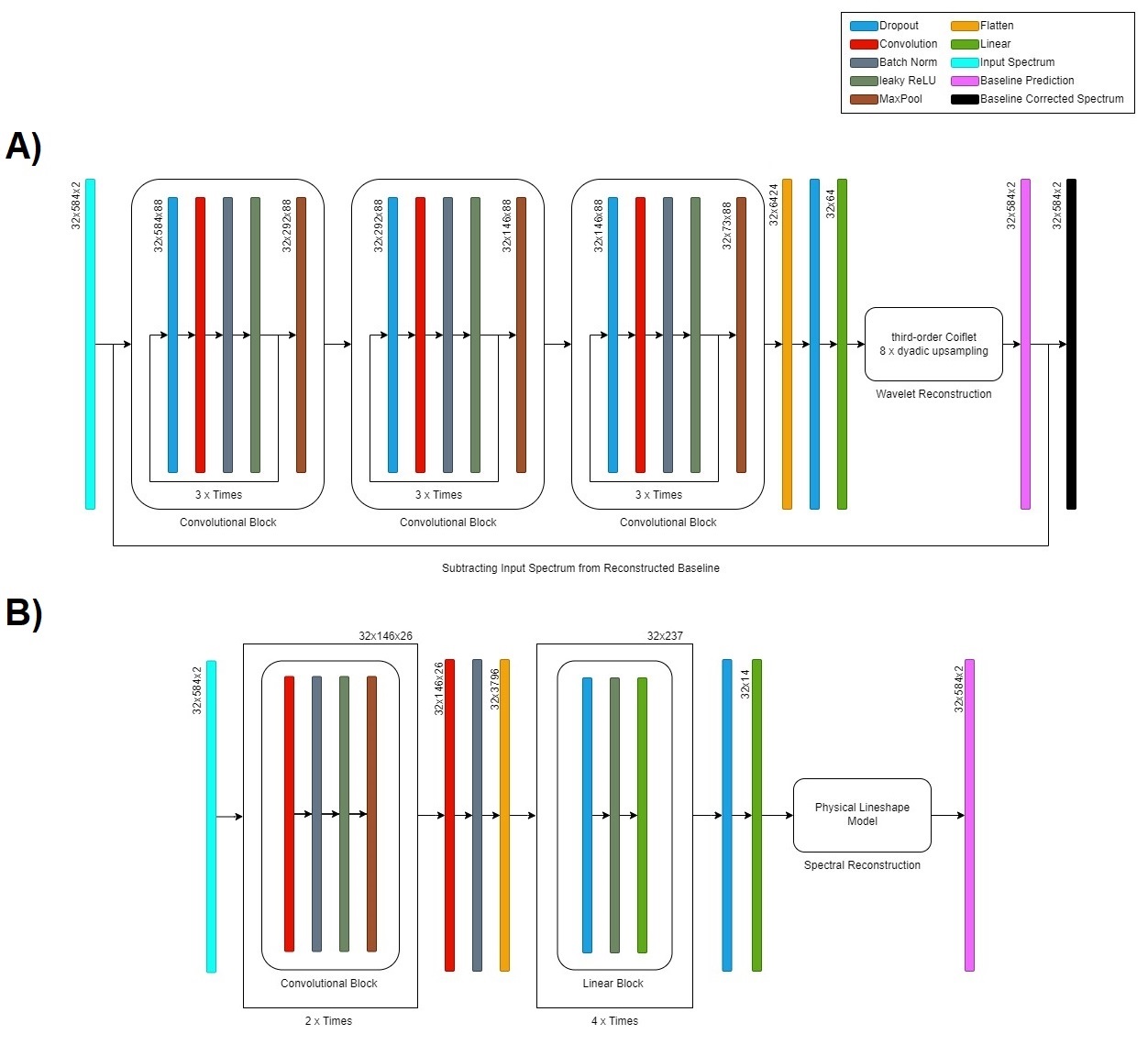
During the course of this project, a convolutional neural Network (CNN) was optimised to process human brain FID-MRSI data. The network takes real and imaginary parts of the spectrum as input. In a first step, the network predicts a set of wavelet parameters, which are being convolved with third-order coiflet filters and dyadically upsampled2 to produce accurate representations for underlying baselines of unknown origin. This process is done separately for real and imaginary components of the spectra. The baseline estimation is used to correct the input data, before consequently estimating metabolite amplitudes and spectral parameters. The resulting prediction parameters are then put into a physical model for spectral reconstruction purposes. Overall, the aim was to achieve robust spectral quantification on simulated 7T magnetic resonance brain spectra over a specific spectral range (4.2-1.8 ppm) with different levels of SNR (6.8-18.2). The network itself was optimized using Adam optimization4, as well as neural architecture search and hyperparameter tuning provided by the Neural Network Intelligence (NNI) package5. A description of the networks final architecture is shown in Fig 1. Furthermore, the network was trained using supervised learning on a mean squared error (MSE) loss function, with leaky rectified linear unit (leakyReLU) activation and Kaiming initialization6. The training data (n = 64.000 spectra) was procedurally generated during individual epochs, while validation (n = 6.400 spectra) and testing (n = 6.400 spectra) was repeatedly performed on the same pre-simulated data to ensure consistency across epochs. The underlying metabolite basis set was generated with the software package jMRUI7, utilizing NMR-SCOPE and QUEST for the quantummechanical simulation of combined creatine and phosphocreatine (tCr=Cr+PCr), glutamate (Glu), glutamine (Gln), N-acetylaspartate (NAA), N-acetylaspartylglutamate (NAAG), combined phosphorylcholine and glycerophosphorylcholine (tCh=PC+GPC), myo-Inositol (mI), taurine (Tau) and γ-aminobutyric acid (GABA). The predicted spectral fitting parameters include zero-order phase (±90 deg), frequency shift (±12 Hz), additional lorentzian and gaussian T2* line broadening constants (0.1-1.0 ms). The acquisition delay was fixed (1.3 ms) for all spectra. Computations were performed using Pytorch8 on four Tesla V100 GPU cards (Nvidia, Santa Clata, CA, US) mounted to a DGX station.Results
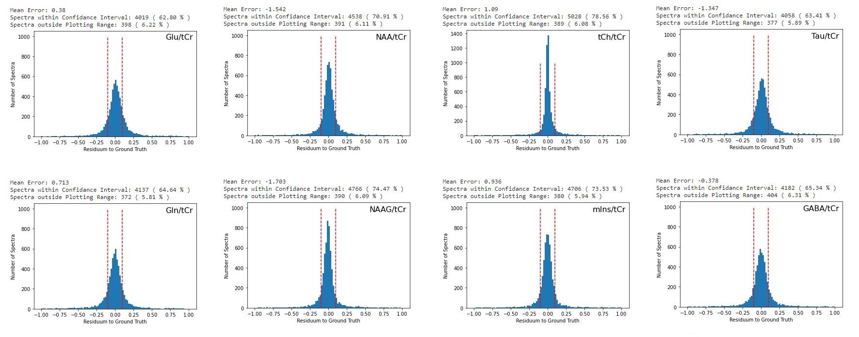
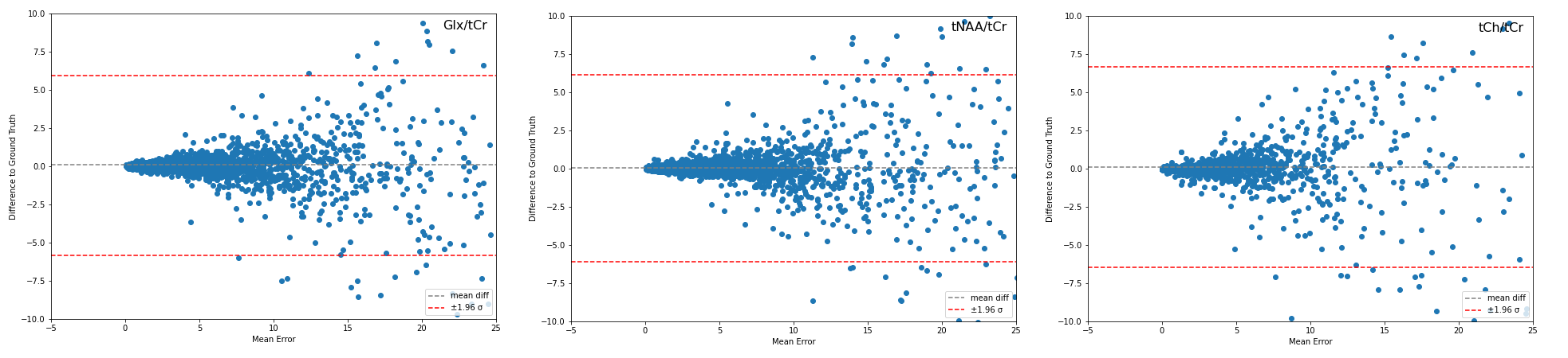
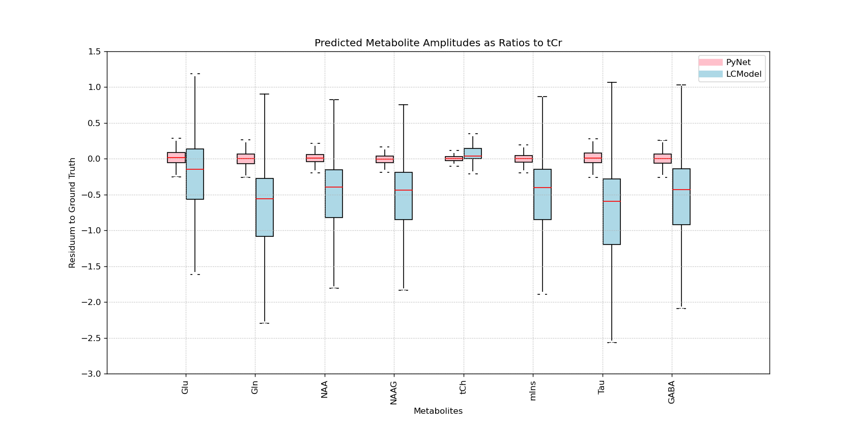
The networks performance on metabolite quantification was compared to LCModel by calculating residue to the ground truth from ratios to tCr for all metabolite amplitudes, shown in Fig 2-4. Excluding heavy outliers from the analysis, we report the following mean errors and standard deviations for the CNN and LCModel approach: Metabolite (CNN; LCModel), Glu (0.022±0.615; -0.323±1.041), Gln (-0.012±0.611; -0.833±1.133), NAA (0.013±0.641; -0.649±1.0156), NAAG (-0.0201±0.589; -0.699±1.015), tCh (0.027±0.639; 0.140±0.785), mIns (-0.004±0.592; -0.675±1.017), Tau (0.016±0.611; -0.908±1.224), GABA (0.003±0.642; -0.702±1.082). Spectral fitting parameters quantified by the CNN show MAE of 6.291±1.911 Hz for frequency shifts, 0.131±0.176 rad for zero-order phase and 7.012±5.445 and 0.007±0.007 ms for lorentzian and gaussian T2* broadening constants respectively. Analysing the testing dataset took the CNN 9 s and LCModel 6240 s, which corresponds to a time difference by the factor of ~700. Sample fitting spectra after reconstruction are given in Fig 5.Discussion
The possibility of combining physical models with means of DL gives rise to improved means of quantification. To ensure optimal performance on in-vivo data in the future, ranges for the simulation and network parameters need to be extended though, by including first-order phase and further baseline variations (macromolecule signals and lipid artifacts). Furthermore, it should be emphasised, that the low accuracy of LCModel on the quantification of simulated spectra should not be seen as a sign for bad performance, but rather indicates that the simulated spectra are not representative enough for in-vivo data and thus might explain the observed underperformance of LCmodel quantification.Conclusion
This project improves the spectral quantification of brain MRS data and shows potential for future whole-brain MRSI (wbMRSI) applications, as the robust CNN approach significantly speeds up quantification times, which brings us closer to MRSI being part of routine clinical practices.Acknowledgements
We acknowledge financial support by the FWF (P34198).References
1. Yamashita et al., Convolutional neural networks: an overview andapplication in radiology. Insights Imaging. 2018;9(1):611-629.
2. Gurbani et al., Incorporation of a spectral model in a convolutional neural network for accelerated spectral fitting. Magnetic Resonance in Medicine. 2019;81(5):3346-3357.
3. Lee et al., Intact metabolite spectrum mining by deep learning in proton magnetic resonance spectroscopy of the brain. Magnetic Resonance in Medicine. 2019;82(1):33-48.
4. Kingma et al., Adam: A Method for Stochastic Optimization. ICLR 2015. 2017(9).
5. Microsoft, Neural Network Intelligence (v2.9). 2022https://github.com/microsoft/nni.
6. Kaiming et al., Delving Deep into Rectifiers: Surpassing Human-Level Performance on ImageNet Classification. 2015 IEEE (ICCV). 2015;1026-1034.
7. Stefan et al., Quantitation of magnetic resonance spectroscopy signals: The jMRUI software package. Measurement Science and Technology. 2009;20(10).
8. Paszke A et al., Automatic differentiation in PyTorch. NIPS-W. 2017.
Figures
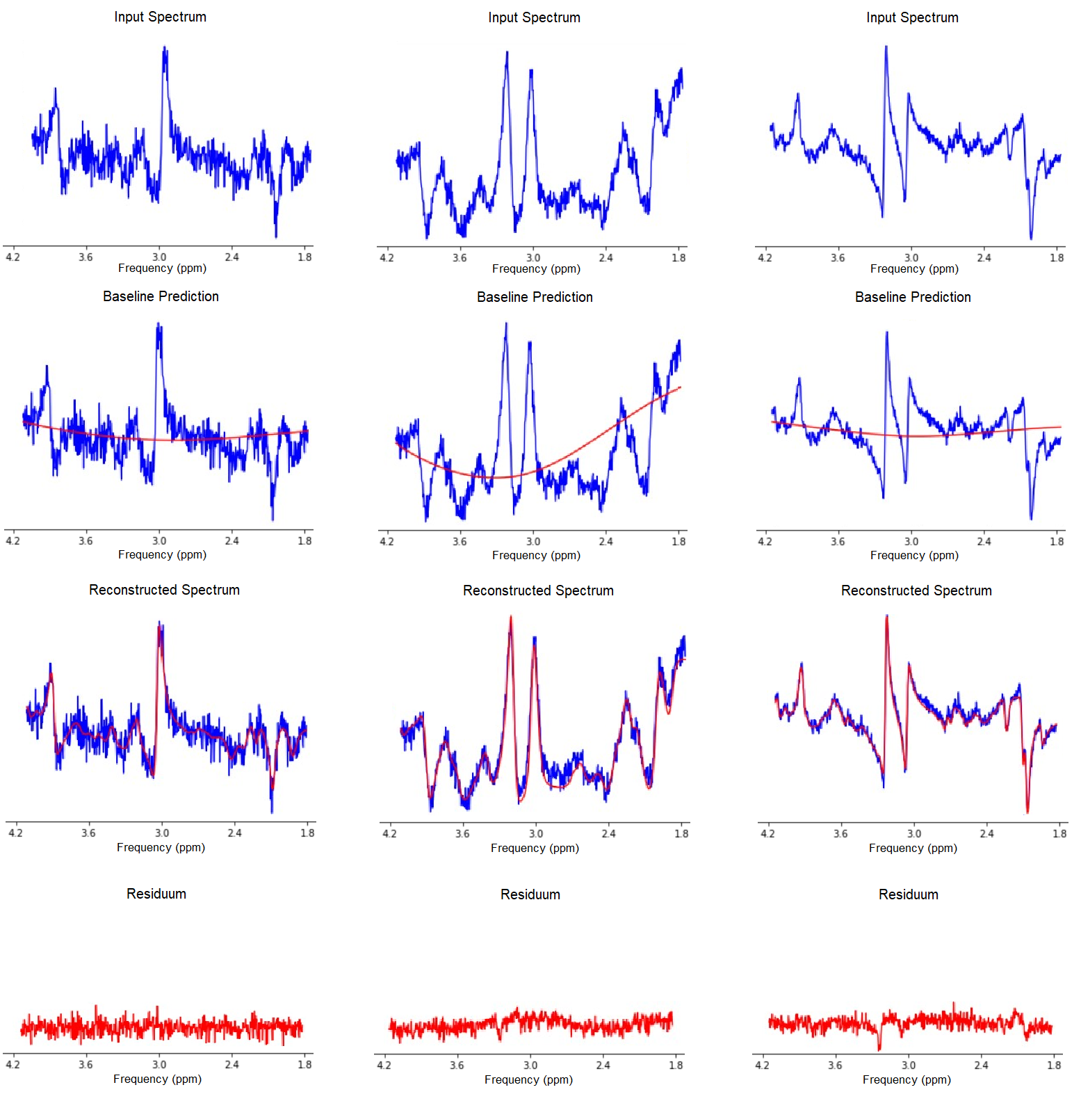
Random sample spectra, selected from the testing-dataset, for visual representation of the reconstruction capabilities of the CNN plotted over the frequency range in ppm. The figure depicts input spectra, corresponding baseline prediction, spectral reconstruction, as well as residue.