3654
Reconstructing 3D Velocity and Pressure Fields From 2D Flow Measurements Using Physics Informed Neural Networks1Institute of Biomedical Engineering, ETH Zurich, Zurich, Switzerland
Synopsis
Keywords: Flow, Velocity & Flow
We propose physics-informed neural networks to augment 2D phase-contrast flow measurements in order to reconstruct full 3D velocity and pressure fields. In this conceptual work, 2D flow measurements are assimilated using the incompressible Navier-Stokes equations defined on the vessel anatomy reconstructed from anatomical scans. The network leverages a low-rank representation of velocity and pressure fields as physical prior and it is demonstrated to reconstruct 3D velocity and pressure gradient fields with good accuracy.
Introduction
Phase-contrast (PC) magnetic resonance imaging (MRI) has enabled measurements of space- and time-resolved blood velocities (4D flow MRI) from which it was possible to associate abnormal flow patterns in different cardiovascular diseases [1]. Despite recent advancements in acquisition and reconstruction protocols [2,3], flow measurements in clinical routine are still affected by limited coverage and resolution, low signal-to-noise ratios and long scanning times. A number of works have addressed the noise reduction and limited spatio-temporal resolution by employing regularizers based on fluid dynamic equations [4-6].We propose to use 2D PC MRI acquisitions coupled with anatomical 3D scans to generate the full 3D flow field in a vessel of interest and reconstruct both velocity and pressure fields. This is achieved using Physics Informed Neural Networks (PINNs) regularized with the partial differential equations governing blood flow. The large computational cost is mitigated by embedding a low-rank representation based on radial bases (RB), which provides a biophysical prior to PINNs predictions. The concept is demonstrated on synthetic geometries representing typical flow conditions.
Methods
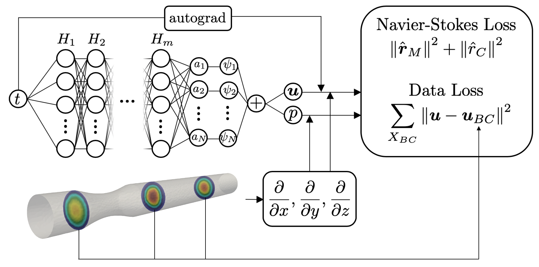
The PINN is designed as a dense neural network whose input is the phase of the cardiac cycle, t, and the outputs are velocity vectors, u, and pressure, p, on the geometry (Fig. 1). The network outputs the amplitudes of the low-rank bases providing the approximation of the velocity vectors and pressure fields, which are reconstructed by the last, non-trainable projection layer. The bases are obtained from a dataset of synthetic simulations using a biophysical model of pulsatile unsteady laminar flow in a cylinder with varying degrees of stenosis. The simulated flow regimes are representative of a lesioned carotid artery branch [7,8]. The RB are obtained by applying Proper Orthogonal Decomposition to the simulated dataset as in [9-11] and are used as bases in the network projection layer.To train the PINN for a specific new case, the cost function derived from the cost associated to the residuals of the partial differential equations (PDE) is minimized (see Navier-Stokes (NS) loss in Fig.1 composed of the momentum, rM, and mass conservation, rc, residuals, see [9] for details on the NS equations) while ensuring consistency of the solution with the measurements uBC (see Data Loss in Fig.1). The calculation of the PDE residual requires to compute the spatial gradients of velocity and pressure fields which follows the approach presented in [10].
To validate our approach, we simulated synthetic MRI measurements on 2D sections along a three-dimensional vessel [11] on 20 test cases not included in the training set. The measurements are corrupted with Gaussian noise and bias values with randomly selected gradients along two directions of the slice planes. Velocity values are then interpolated on the mesh points of the vessel and used as uBC in the data loss term of the training function.
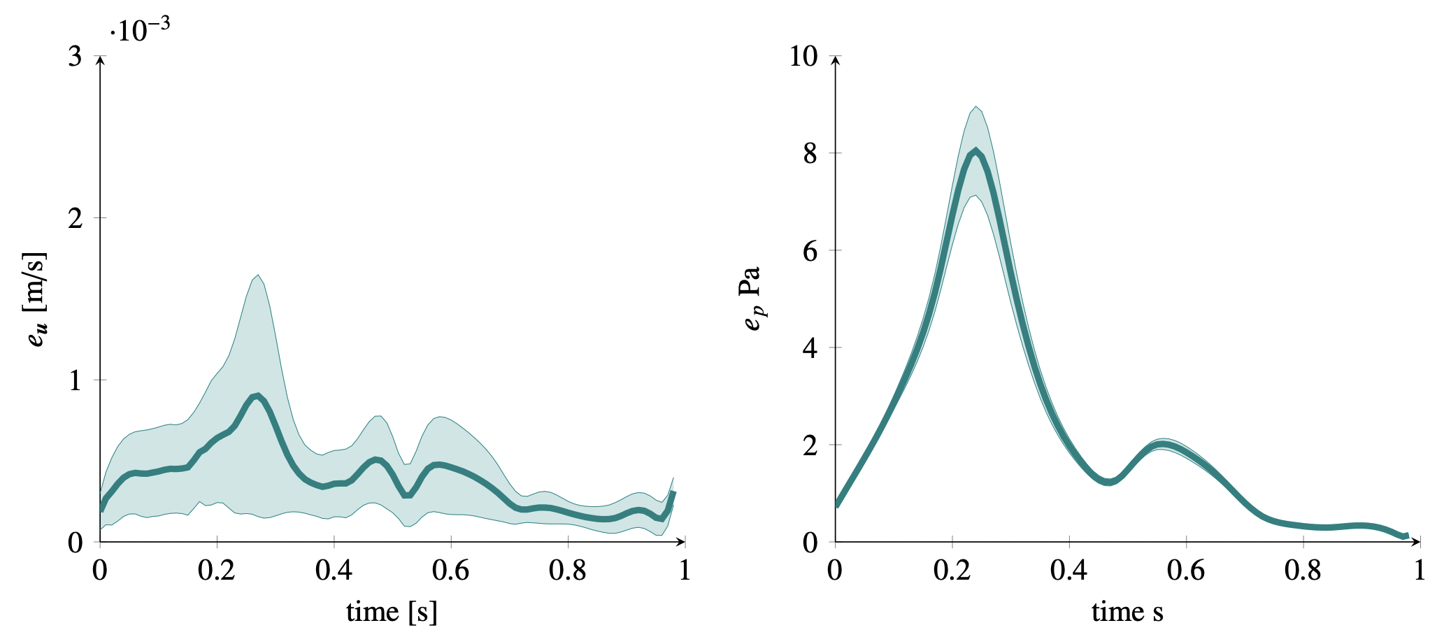
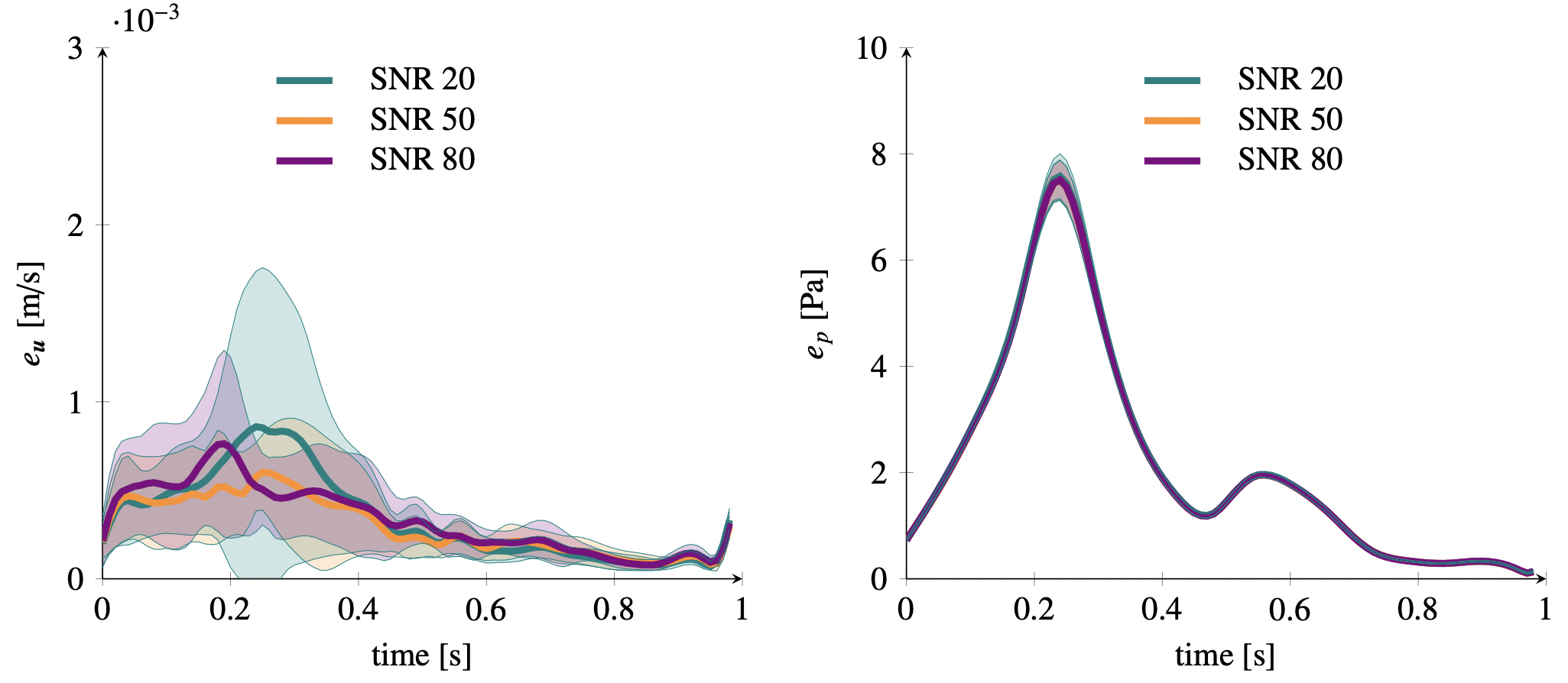
The PINN performance on the test cases is quantified using the anatomy-averaged absolute errors of velocity, eu = ||uGT-uPINN||2, and pressure, ep = ||pGT-pPINN||2 where the subscripts GT and PINN refer to the reference solution, computed with a biophysical model, and to PINN predictions, respectively.
Results
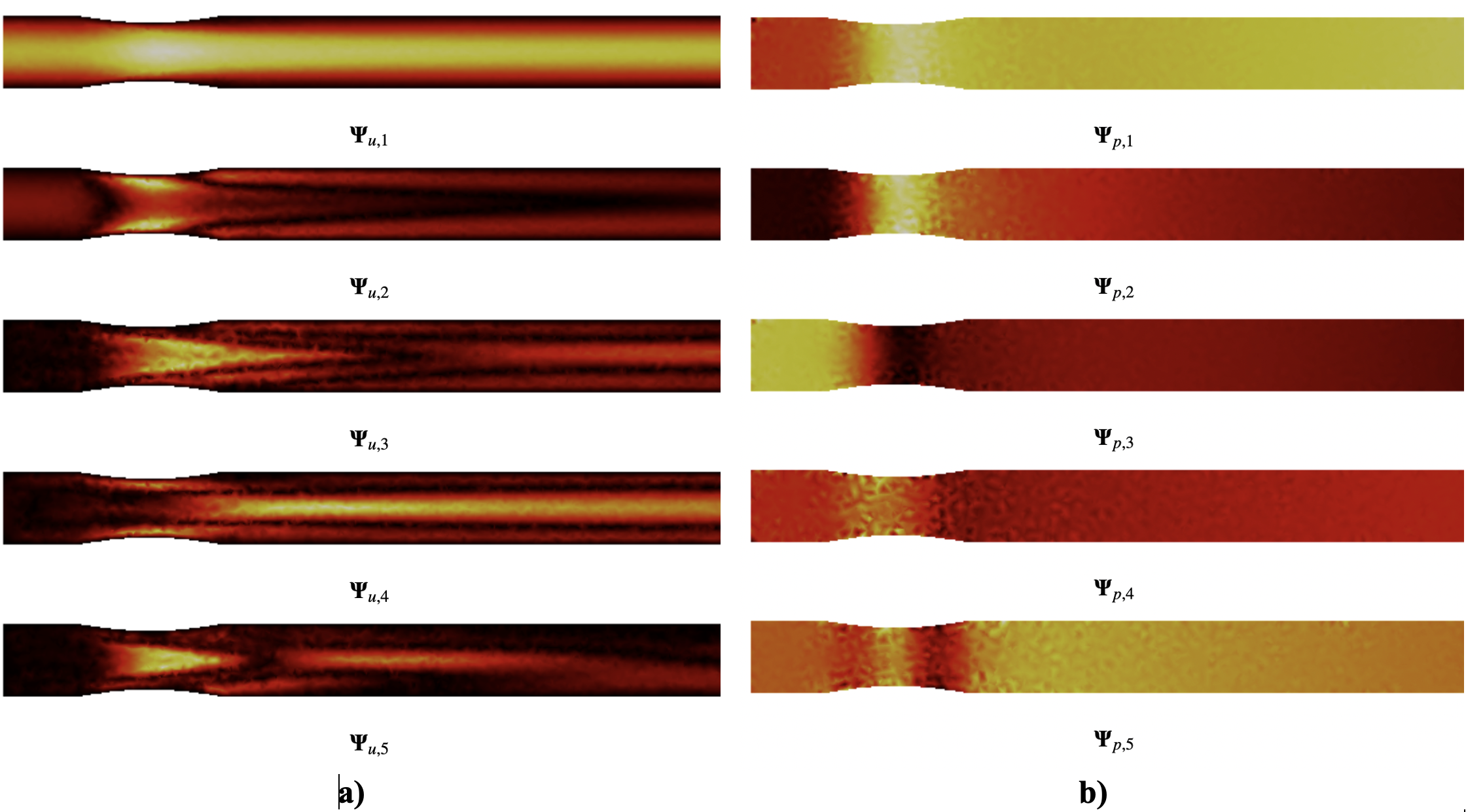
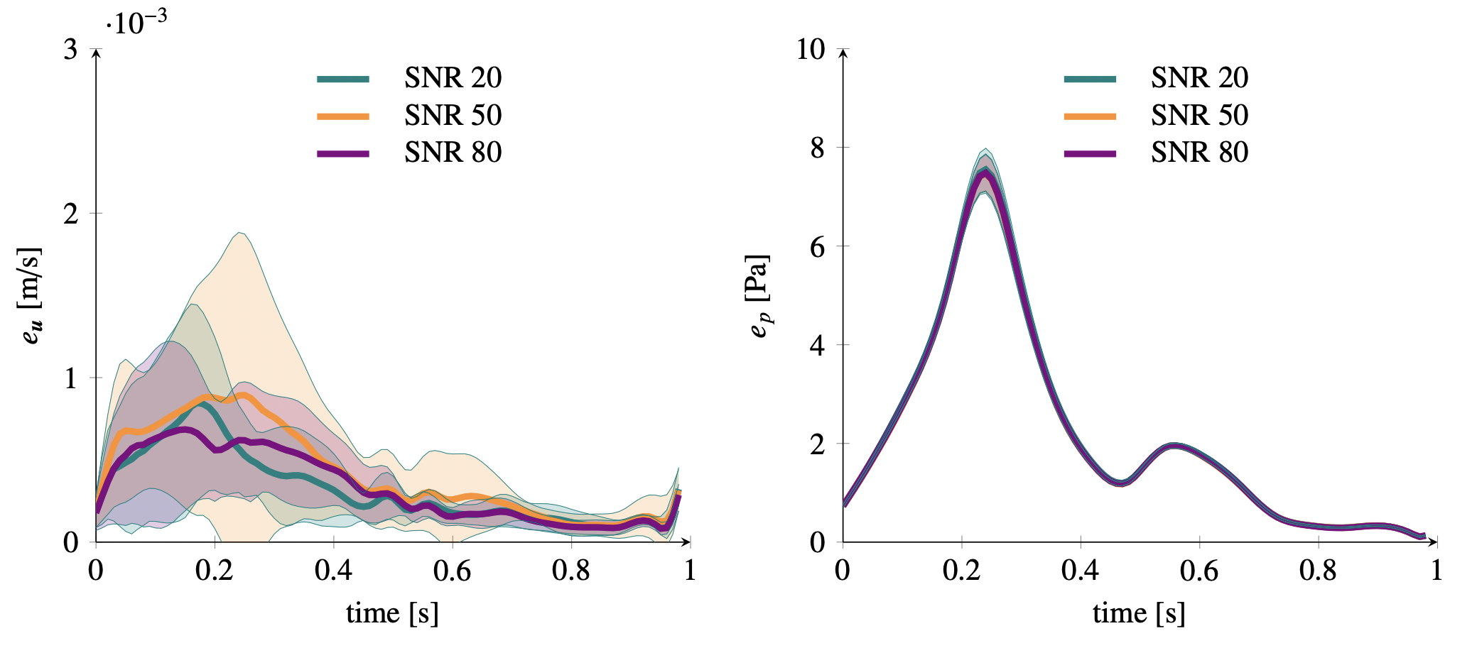
Figure 2 shows the 5 bases of the low rank representation for velocity (2.a) and pressure (2.b) used in the last-non trainable PINN layer. Fig. 3 plots the errors over the pulsatile cycle of PINN predictions against the reference model for velocity (a) and pressure (b) when using the exact values of flow at inlet velocity as measurement data uBC. The largest errors are observed at peak systole with mean (standard deviation) value of 10-3 (7 ×10⁻⁴) m/s and 8(0.1) Pa for velocity and pressure, respectively. Figure 3 and 4 show the errors when using the synthetic MRI measurements without and with bias for SNR values of 20,50 and 80. Similar errors are observed in all these cases, with magnitude comparable to those of the noiseless cases (Figure 3).Discussion
We have demonstrated that by using Physics Informed Neural Networks it is possible to augment 2D PC MRI measurements and to reconstruct the full pulsatile velocity and pressure fields in the vessel of interest. The method is robust to Gaussian noise and to artificial biases added to the simulated MRI measurements. The computational cost of this approach is an order of magnitude lower than conventional approaches where an optimization problem based on the Navier-Stokes equations is used. Particularly, on a cpu, training the PINN for one case takes approximately 10 minutes, and allows for real time predictions afterwards, while a conventional simulation takes approximately 2 hours. This is mainly achieved using the low-rank representation as physical prior to the PINN prediction. In this scenario, 2D PC MRI measurements covering only 10% of the total vessel volume with high spatial and temporal resolution could be used reconstruct the full field in vessels of interest, significantly reducing scanning time.Acknowledgements
The authors acknowledge the financial support of the SwissNational Science Foundation (SNF) [grant CR23I3-166485]References
[1] Markl, M., Frydrychowicz, A., Kozerke, S., Hope, M., Wieben, O., 2012. 4D flow MRI. Journal of Magnetic Resonance Imaging 36, 1015–1036. doi:doi.org/10.1002/jmri.23632
[2] Walheim, J., Dillinger, H., Gotschy, A., Kozerke, S., 2019. 5D flow tensor MRI to efficiently map Reynolds stresses of aortic blood flow in-vivo. Scientific Reports 9, 18794. doi:10.1038/s41598-019-55353-x.
[3] Vishnevskiy, V., Walheim, J., Kozerke, S., 2020. Deep variational network for rapid 4D flow MRI reconstruction. Nature Machine Intelligence 2, 228–235. doi:10.1038/s42256-020-0165-6.
[4] Busch, J., Giese, D., Kozerke, S., 2017. Image-based background phase error correction in 4D flow MRI revisited. Journal of Magnetic Resonance Imaging 46, 1516–1525. doi:doi.org/10.1002/jmri.25668.
[5] Vlasenko, A., Schnorr, C., 2010. Physically consistent and efficient variational denoising of image fluid flow estimates. IEEE Transactions on Image Processing 19, 586–595. doi:10.1109/TIP.2009.2036673.
[6] Rispoli, V.C., Nielsen, J.F., Nayak, K.S., Carvalho, J.L.A., 2015. Computational fluid dynamics simulations of blood flow regularized by 3D phase contrast MRI. BioMedical Engineering OnLine 14. doi:10.1186/s12938-015-0104-7.
[7] Krejza, J., Arkuszewski, M., Kasner, S.E., Weigele, J., Ustymowicz, A., Hurst, R.W., Cucchiara, B.L., Messe, S.R., 2006. Carotid artery diameter in men and women and the relation to body and neck size. Stroke 37, 1103–1105. doi:10.1161/01.STR.0000206440.48756.f7.
[8] Likittanasombut, P., Reynolds, P., Meads, D., Tegeler, C., 2006. Volume flow rate of common carotid artery measured by doppler method and color velocity imaging quantification (CVI-Q). Journal of Neuroimaging 16, 34–38. doi:https://doi.org/10.1177/1051228405001523.
[9] Buoso, S., Joyce, T., Kozerke, S., 2021. Personalising left-ventricular biophysical models of the heart using parametric physics-informed neural networks. Medical Image Analysis , 102066. doi.org/10.1016/j.media.2021.102066
[10] Buoso, S., Manzoni, A., Alkadhi, H., Kurtcuoglu, V., 2022. Stabilized reduced-order models for unsteady incompressible flows in three-dimensional parametrized domains. Computer and Fluids, 246, 105604. 10.1016/j.compfluid.2022.105604
[11] Buoso, S., Manzoni, A., Alkadhi, H., Plass, A., Quarteroni, A., Kurtcuoglu,V., 2019. Reduced-order modeling of blood flow for noninvasive functional evaluation of coronary artery disease. Biomechanics and Modeling in Mechanobiology 18, 1867–1881. doi:10.1007/s10237-019-01182-w.
[12] Dirix P, Buoso S, Pepper ES and Kozerke S (2022), ‘Synthesis of patient-specific multipoint 4D flow MRI data of turbulent aortic flow downstream of stenotic valves’, Scientific Reports, 12, 16004. 10.1038/s41598-022-20121-x
Figures