3646
On the interplay of encoding and readout in turbulent flow imaging
Charles McGrath1, Pietro Dirix1, Jonathan Weine1, and Sebastian Kozerke1
1University and ETH Zurich, Zurich, Switzerland
1University and ETH Zurich, Zurich, Switzerland
Synopsis
Keywords: Flow, Velocity & Flow, Turbulence
The accuracy of turbulent flow quantification using phase-contrast MRI depends on both the turbulence energy spectrum to be imaged and the sampling spectrum of the velocity encoding gradients. In the present work their interplay is studied in detail, revealing erroneous quantification of intravoxel standard deviation and turbulent kinetic energy in particular in cases exhibiting low turbulence frequencies. It is concluded that experimental design for turbulent flow quantification needs to consider the joint effect of velocity encoding and imaging gradients.
Keywords: Turbulence, TKE, Phase Constrast, Simulation, Flow, Cardiovascular
Introduction
The presence of turbulent blood flow downstream of aortic stenoses1 is linked to various cardiovascular diseases2, hinting at the significance of understanding and modeling of turbulence quantification using MRI3,4.Recent work has indicated the importance of the interaction between the turbulence energy spectra and the sampling spectra of the encoding gradient5. Specifically, when the spectral sampling behavior is not considered, errors can occur in the turbulent kinetic energy (TKE) estimation.
While the design of dedicated gradient waveforms for turbulence flow encoding is well understood, the additional effect of imaging gradients has been considered negligible. Due to the spectral sampling behavior of turbulence encoding, encoding gradient and imaging gradients interact and hence complex changes in sampling spectra can occur. A similar effect has been investigated in the context of diffusion imaging6, concluding that these effects should be considered when readout and encoding gradients have similar strengths.
In this work, we investigate the effect of the readout gradient on the effective sampling spectra and demonstrate its impact using simulated TKE images.
Methods
Brief Turbulence TheoryThe effective signal loss due to dephasing from turbulence can be formulated as5$$\alpha(t)=\frac{\int_{-\infty}^{\infty}D(\omega)S(\omega,t)d\omega}{\int_{-\infty}^{\infty}D(\omega)d\omega},\;\;\;\;[1]$$where $$$t$$$ is the time at which the effect of dephasing is evaluated, $$$\omega$$$ is frequency, $$$\alpha(t)$$$ acts as an exponential damping term ($$$e^{-\alpha(t)}$$$) on the signal, $$$(d\omega)$$$ is the turbulent energy spectrum and $$$S(\omega,t)$$$ is the gradient sampling spectrum, defined as$$S(\omega,t)=|\tilde{q}(\omega,t)|^2,\;\;\;\;[2]$$$$\tilde{q}(\omega,t)=\int_{0}^{t}q(t')e^{i{\omega}t'}dt',{\;\;\;\;}q(t)=\gamma\int_{0}^{t}G(t')dt',\;\;\;\;[3,4]$$where $$$\tilde{q}(\omega,t)$$$ is the Fourier transform of the integral of the encoding gradient $$$G(t)$$$ and $$$\gamma$$$ is the gyromagnetic ratio. As such, the choice of end point $$$t$$$ is important and the addition or removal of gradients will change the spectral shape and hence dephasing $$$\alpha(t)$$$ due to turbulence.
For turbulence estimation the intra-voxel standard deviation (IVSD) is often measured, which is retrieved from the ratio of two images with different flow encoding moment $$$k_{v1}$$$ and $$$k_{v2}$$$ using7$$\sigma_{IVSD}=\sqrt{\frac{2ln(\frac{|S(k_{v2})|}{|S(k_{v1})|})}{k_{v1}^2-k_{v2}^2}},\;\;\;\;[5]$$where $$$k_v=\frac{M_1}{\gamma}$$$ and $$$M_1=\int_{0}^{t}G(t')t'dt'$$$. Alternatively, TKE can be estimated as $$$TKE\:{\propto}\:\sigma_{IVSD}^2$$$.
Simulation Methods
We performed Bloch simulations of a spoiled gradient echo in a stenotic U-bend (70% area stenosis) incorporating turbulent particle tracking using the CMRsim package (https://people.ee.ethz.ch/~jweine/cmrsim/latest/index.html)(see table 1 for parameters). Based on the Langevin equation8,9, particle position updates per step can be formulated as$$\vec{\boldsymbol{x}}_{t+dt}=\vec{\boldsymbol{x}}_t+(\vec{\boldsymbol{U}}_t+\vec{\boldsymbol{u}}_t)dt,\;\;\;\;[6]$$$$\vec{\boldsymbol{u}}_t=\vec{\boldsymbol{u}}_{t-dt}e^{-\frac{dt}{\tau}}+\vec{\boldsymbol{\zeta}}\sqrt{1-e^{-2\frac{dt}{\tau}}},\;\;\;\;[7]$$where $$$\vec{\boldsymbol{x}}$$$ is the particle position, $$$\vec{\boldsymbol{U}}$$$ is the mean velocity, $$$\vec{\boldsymbol{u}}$$$ is the fluctuating velocity, $$$\vec{\boldsymbol{\zeta}}$$$ is a random Gaussian sample from the Reynolds stress tensor, and $$$\vec{\boldsymbol{\tau}}$$$ is the Lagrangian time.
Lagrangian time $$$\tau$$$ was either kept spatially constant or scaled according to the inverse of the spatially predefined TKE, with the defined Lagrangian time corresponding to the 90th spatial percentile.
In order to investigate the effects of gradient inversion and its interaction with the turbulence spectrum, the Lagrangian time was varied between 0.25 and 4ms. As a surrogate for total TKE in the encoded direction, the spatial sum of each image was taken, and the ratio due to gradient inversion was calculated for each Lagrangian time.
Results and Discussion
Figure 2a shows the effect of incorporating the Langevin equation into particle tracking. Figure 2b shows a set of example turbulence spectra for different Lagrangian times $$$\tau$$$.The effect of gradient inversion on both the sampling spectra and the resulting images can be seen in Figure 3, with additional images for varying Lagrangian times shown in Figure 4.
Figure 5 shows the ratio of the summed TKE estimation between inverted and non-inverted gradients, calculated based on the images in Figure 4.
When not considering the readout gradient, inversion has no effect on the sampling spectra. However, when including the readout gradient up to the echo time, the spectra differ noticeably, seen in Figure 3b, which is reflected in the simulated images in Figure 3c-d.
The difference in the resulting turbulence images can be attributed to the redistribution of encoding strength to different regions of the frequency spectra and is thus strongly dependent on the turbulence spectra itself, clearly seen in both Figure 4 and 5. For decreasing Lagrangian time, resulting images converge due to the turbulence spectrum’s flat region fully encompassing the sampling spectra , resulting in equivilent encoding strengths. At longer Lagrangian times, the redistributed gradient spectra sample different regions of the turbulence spectrum, resulting in differing encoding strengths. These image-based results match the expectations from theory. When Lagrangian time is spatially varying, the simulated results show larger deviations from the expected value due to spatial mixing and particle migration.
Additionally, the agreement between image-based ratios and theory in Figure 5 serves as a step toward verification of the turbulence pipeline implemented in the CMRsim framework.
Finally, while this work focused on the effect of the readout gradient, it can be expanded to include all sequence and slice select gradients .
Conclusion
We have investigated the effect of inverting bipolar encoding gradients on turbulence quantification and compared theory with simulation results. Our results show that including the readout gradient influences the velocity-encoding spectra, which in cases exhibiting low turbulence frequencies can result in erroneous turbulence estimation.Acknowledgements
References
- Garcia J, Barker AJ, Markl M. The role of imaging of flow patterns by 4D flow MRI in aortic stenosis. JACC: Cardiovascular Imaging. 2019 Feb;12(2):252-66.
- Ha H, Ziegler M, Welander M, Bjarnegård N, Carlhäll CJ, Lindenberger M, Länne T, Ebbers T, Dyverfeldt P. Age-Related Vascular Changes Affect Turbulence in Aortic Blood Flow. Front Physiol. 2018 Jan 25;9:36.
- Dillinger H, Walheim J, Kozerke S. On the limitations of echo planar 4D flow MRI. Magnetic Resonance in Medicine. 2020 Oct;84(4):1806-16.
- Dirix P, Buoso S, Peper ES, Kozerke S. Synthesis of patient-specific multipoint 4D flow MRI data of turbulent aortic flow downstream of stenotic valves. Scientific reports. 2022 Sep 26;12(1):1-1.
- Dillinger H, McGrath C, Guenthner C, Kozerke S. Fundamentals of turbulent flow spectrum imaging. Magn. Reson. Med. 2021:223–249 doi: 10.1002/mrm.29001.
- Güllmar D, Haueisen J, Reichenbach JR. Analysis of b-value calculations in diffusion weighted and diffusion tensor imaging. Concepts Magn. Reson. Part A Bridg. Educ. Res. 2005;25:53–66 doi: 10.1002/cmr.a.20031.
- Dyverfeldt P, Sigfridsson A, Kvitting JPE, Ebbers T. Quantification of intravoxel velocity standard deviation and turbulence intensity by generalizing phase-contrast MRI. Magn. Reson. Med. 2006;56:850–858 doi: 10.1002/mrm.21022.
- Huilier DGF. An overview of the lagrangian dispersion modeling of heavy particles in homogeneous isotropic turbulence and considerations on related LES simulations. Fluids 2021;6 doi: 10.3390/fluids6040145.
- Dehbi A. Turbulent particle dispersion in arbitrary wall-bounded geometries: A coupled CFD-Langevin-equation based approach. Int. J. Multiph. Flow 2008;34:819–828 doi: 10.1016/j.ijmultiphaseflow.2008.03.001.
Figures
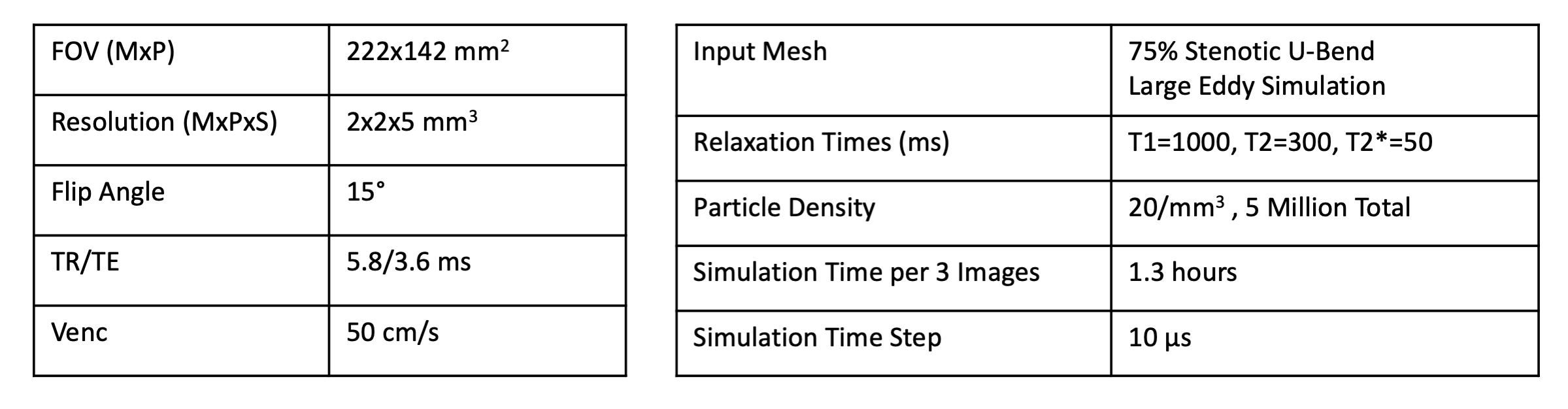
Figure 1: Table of acquisition parameters and simulation parameters
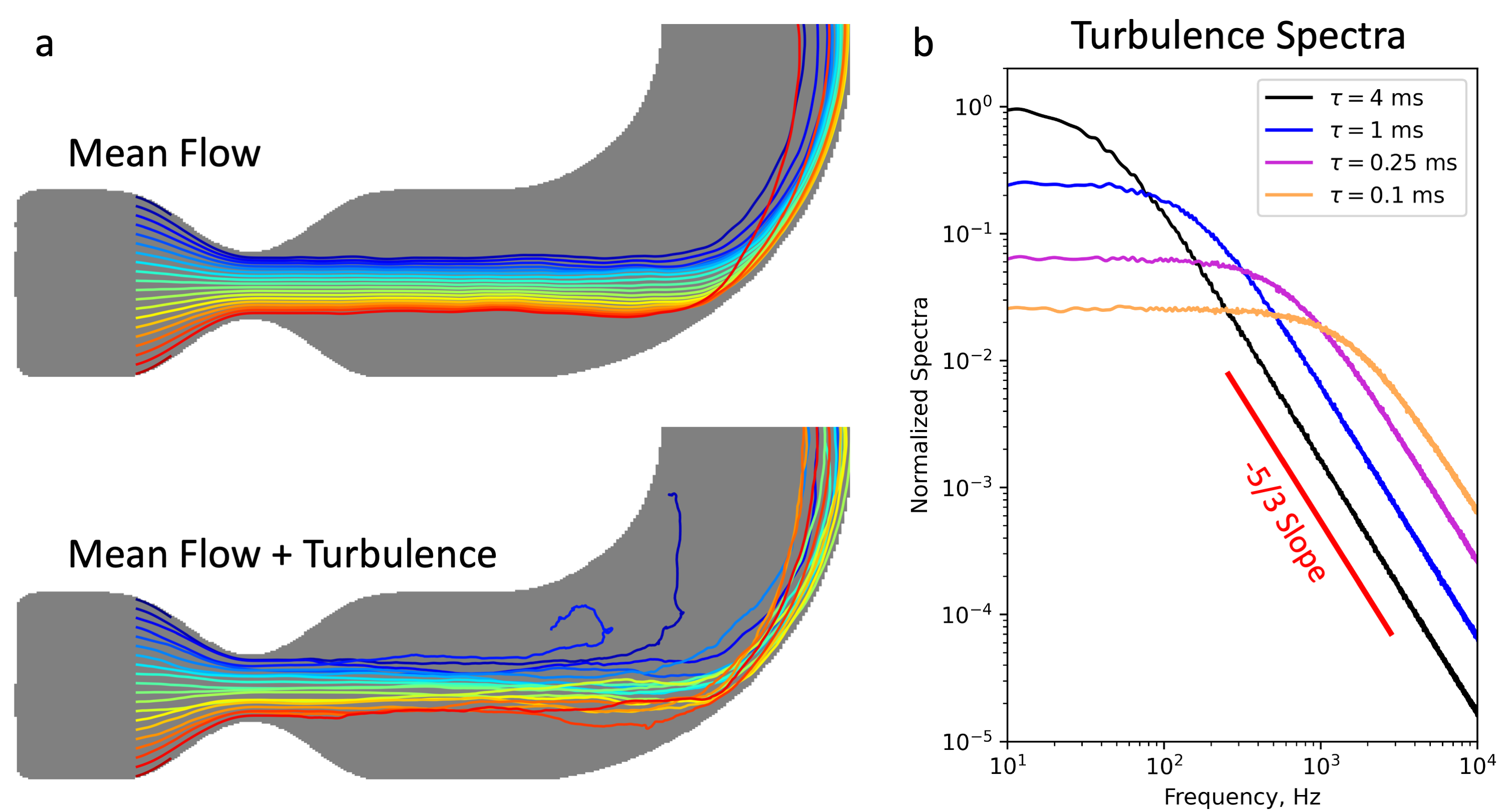
Figure 2: (a) Comparison of particle trajectories generated with mean flow only (top) and with Langevin turbulent trajectories (bottom) for a 70% stenotic U-Bend. Flow fields are generated using large eddy simulation. (b) Simulated turbulence spectra generated by Langevin tracking for varying Lagrangian times. Spectra transition between a flat region to a region of -5/3 slope at a frequency dependent on the Lagrangian time.
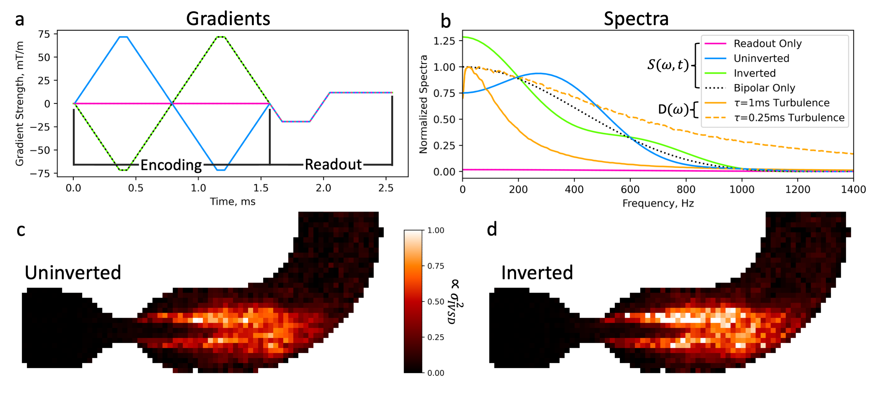
Figure 3: Encoding gradients as well as readout gradient (a) and their corresponding sampling spectra (b). Also shown in (b) are the turbulence spectra corresponding to a Lagrangian times of 1ms and 0.25ms. (c) and (d) show the estimate for the un-inverted and inverted cases. These are estimated $$$\sigma_{IVSD}^2$$$ based on equation 5, with the second encoding with $$$M_1=0$$$ (readout only case in a-b). A clear effect of inverting the encoding gradient can be seen.
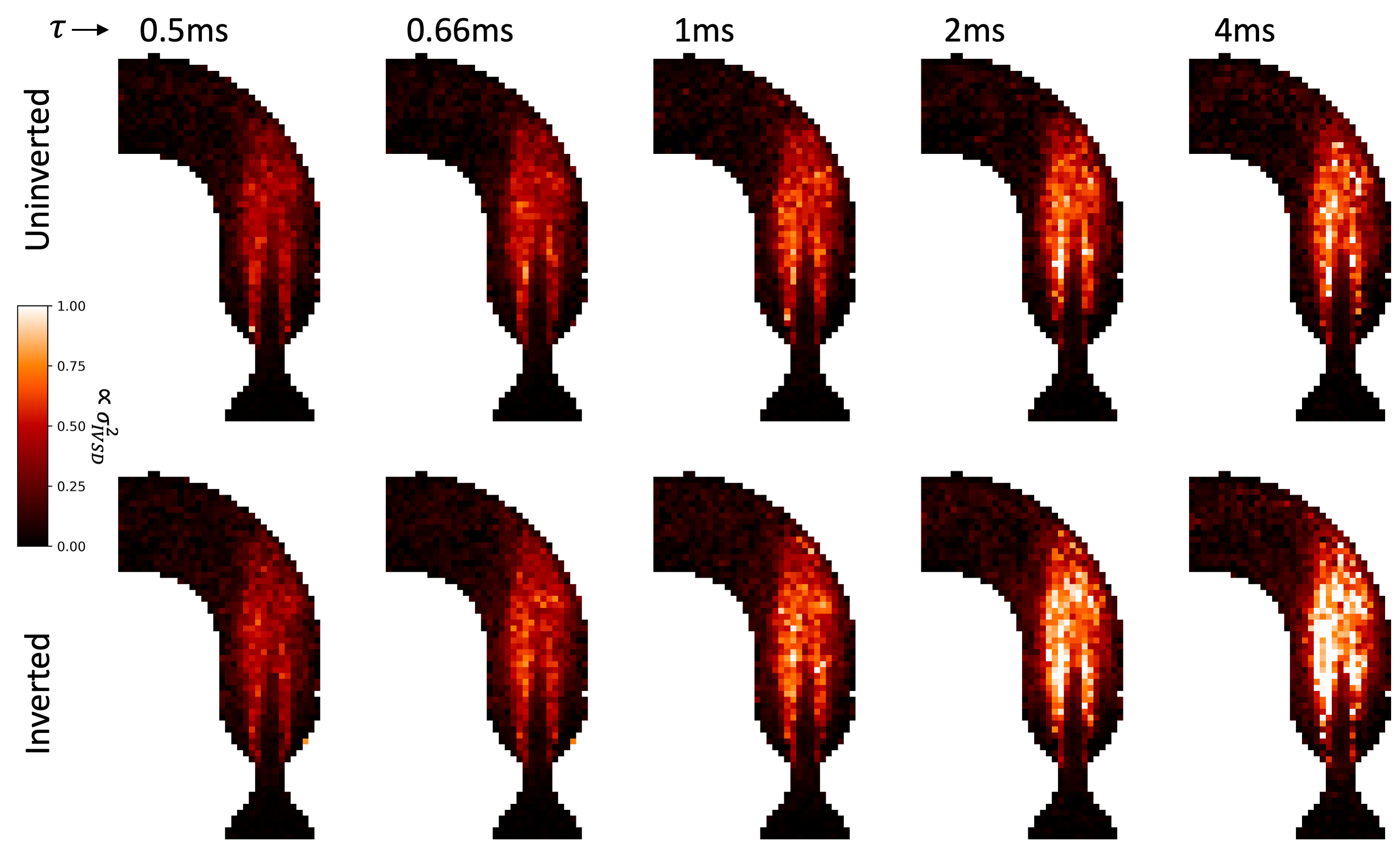
Figure 4: Simulated $$$\sigma_{IVSD}^2$$$ images for a range of Lagrangian times and for both un-inverted and inverted velocity encoding gradients. For short Lagrangian times, inversion of velocity encoding gradients has minimal effect, however as Lagrangian time increases the two gradient cases deviate.
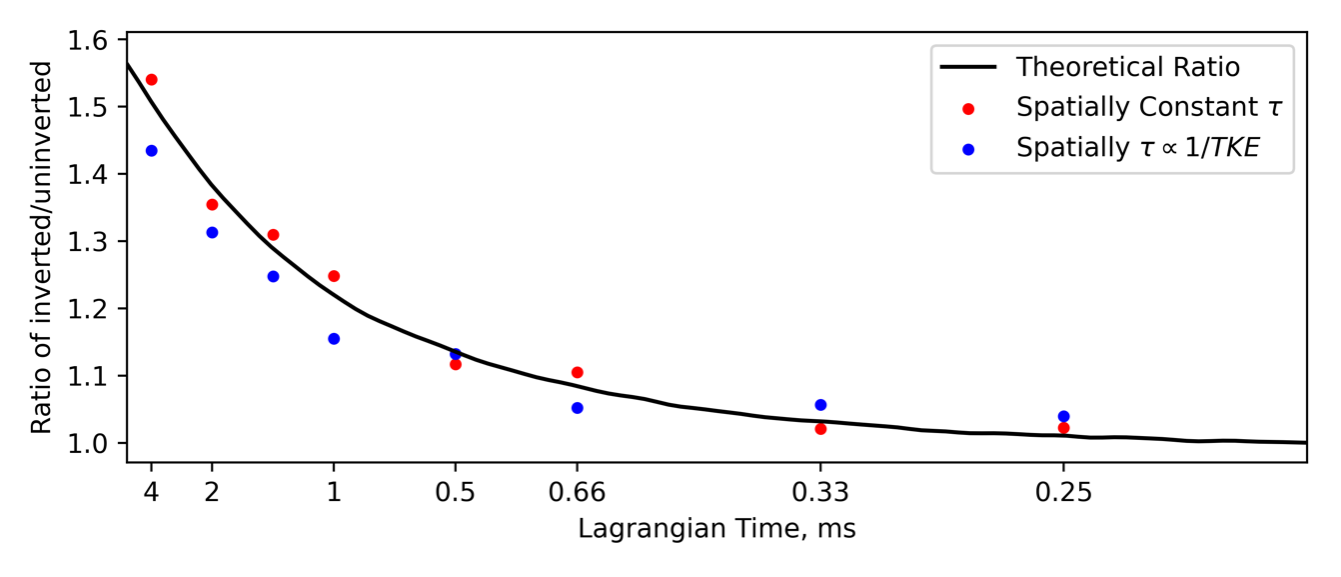
Figure 5: Plot of the ratio of total TKE estimated between inverted and uninverted gradient, showing the factor by which total TKE changes due to encoding gradient inversion. Specifically, each point is given by $$$\frac{\Sigma \sigma_{IVSD}^2[inverted]}{\Sigma \sigma_{IVSD}^2[uninverted]}$$$ for a given Lagrangian time. Two cases are shown, spatially constant Lagrangian time and spatially varying Lagrangian time based on 1/TKE. Also shown is the expected ratio calculated by solving equation 1 directly using the spectra shown in Figures 2 and 3.
DOI: https://doi.org/10.58530/2023/3646