3631
Accelerating 2D Kidney Magnetic Resonance Fingerprinting using Deep Learning–Based Tissue Quantification
Huay Din1, Christina J. MacAskill2, Sree Harsha Tirumani2,3, Pew-Thian Yap4, Mark Griswold2,3, Chris Flask2,3, and Yong Chen1,3
1Case Western Reserve University, Cleveland, OH, United States, 2Department of Radiology, Case Western Reserve University, Cleveland, OH, United States, 3Department of Radiology, University Hospitals Cleveland Medical Center, Cleveland, OH, United States, 4Department of Radiology, University of North Carolina at Chapel Hill, Chapel Hill, NC, United States
1Case Western Reserve University, Cleveland, OH, United States, 2Department of Radiology, Case Western Reserve University, Cleveland, OH, United States, 3Department of Radiology, University Hospitals Cleveland Medical Center, Cleveland, OH, United States, 4Department of Radiology, University of North Carolina at Chapel Hill, Chapel Hill, NC, United States
Synopsis
Keywords: Kidney, Quantitative Imaging, Cancer
In this pilot study, we developed and optimized a spatially-constrained convolutional neural network to accelerate the scan time for 2D kidney Magnetic Resonance Fingerprinting (MRF). Our results suggest that an acceleration factor of 3 can be achieved with the proposed method, which shortens the 2D breath-hold MRF scan from 15 sec to 5 sec. In addition, the deep learning based approach can be applied for T1 and T2 quantification of both normal renal tissues and pathologies including renal cell carcinoma.Introduction
Magnetic Resonance Fingerprinting (MRF) is a new quantitative MR imagine technique, which can provide rapid and simultaneous quantification of multiple tissue properties (1). Recently, deep learning based methods have been integrated with MRF to further improve its speed for both 2D and 3D acquisitions (2, 3). However, most of these studies are focused on stationary brain imaging, where its utility in quantitative abdominal imaging has not been widely explored. Application of the MRF method in these organs faces more technical challenges due to respiratory motions (4). In addition, most of the deep learning methods are tested with MRF measurement obtained from normal tissues and its applicability in characterization of abnormal tissues has not been evaluated. The objectives of this pilot study are to 1) develop and optimize a spatially-constrained convolutional neural network (CNN) to accelerate 2D kidney MRF acquisition (5) and 2) evaluate its capability in quantitation of T1 and T2 relaxation times for renal cell carcinoma (RCC).Methods
All imaging was performed on a Siemens 3T MR scanner (Skyra or Vida). The kidney MRF data was acquired using a FISP-based sequence with a FOV of 40×40 cm, matrix size of 256×256 and slice thickness of 5 mm (4). A total of 1728 MRF time frames were acquired in a single breath-hold of ~15 seconds. Kidney MRF dataset was acquired from 45 subjects. These included 22 normal volunteers and 23 patients with a variety of pathologies such as RCC, autosomal recessive polycystic kidney disease (ARPKD), and cystic fibrosis (CF). An average of 3~5 slices were acquired from each subject, yielding a total of 147 slices from all the subjects for the training and testing purposes.A UNet-based, spatially constrained CNN with residual channel attention was adopted and optimized to retrospectively accelerate 2D kidney MRF acquisition (5). The original deep learning method was developed for high-resolution 2D brain MRF. To adapt for quantitative kidney imaging, multiple network parameters were optimized, including the learning rate policy, patch size and batch size settings. To test whether patient data is needed in the training process, two different training sets were used, including 1) MRF dataset only obtained from normal subjects and 2) dataset obtained from a mixture of normal subjects and patients with pathologies (RCC, ARPKD, and CF). Additionally, to evaluate the performance of deep learning methods in characterizing pathologies, testing dataset was designed to contain data acquired from both normal subjects and patients with different grades of RCC (benign, low-grade and high-grade tumors).
Results
Two different learning rate policies were evaluated, including a ramped learning rate policy and an on-demand policy. For the latter, the learning rate was updated dynamically as the network progressed in the training (Fig 1). Our results show that both the ramped and on-demand learning rates converged to similar minimum loss, but the on-demand policy produced more stable loss curves and converged faster during the training process. We further evaluated network performance with respect to batch and patch sizes. The lowest RMSE values for T1 and T2 quantification were achieved with a batch size of 8 and patch size of 64 for 2D kidney MRF (Fig 2).With the optimized network settings, we further applied the method to retrospectively accelerate kidney MRF with 3x and 4x undersampling, corresponding to tissue mapping using only 576 and 432 time points, respectively. Fig 3 shows that the network trained with patient scans provides slight improvement in comparison to the network trained with normal subjects alone. Fig. 4 shows representative MRF T1 and T2 maps obtained from a normal subject using 576 time points. Our results show that deep learning techniques can achieve 3x acceleration along the temporal dimension while providing accurate and high-quality T1 and T2 maps of the kidney.
We further evaluated the developed method in quantification of T1 and T2 relaxation times for various subtypes of RCCs, including benign, low-grade and high-grade tumors. The evaluation was performed with 3x acceleration and the results were compared with the reference values obtained with full MRF dataset. As shown in Fig 5, the proposed method provides comparable map quality as the reference results using only one third of the MRF data, which corresponds to a short 5-sec MRF scan. Lower T1 and T2 values were observed for the low-grade RCC case, which in general presents the highest T1 and T2 values. However, no evident differences were noticed for the results with the two training dataset containing patient scans or not.
Discussion and Conclusion
In this study, we evaluated the utility of deep-learning-based tissue mapping for accelerating 2D kidney MRF method. At least 3x acceleration can be achieved, which largely reduces the current 2D kidney MRF scan from 15 sec to only 5 sec, rendering a more comfortable breath-hold that is feasible for most of patients. Our results also suggest that the proposed method can be applied for quantitative T1 and T2 characterization of both normal and abnormal tissues in kidney imaging. Future work will be performed to optimize both MRF acquisition pattern and network structure to further improve its quantification accuracy, especially for tissue components with prolonged relaxation times.Acknowledgements
Our group receives research support from Siemens Healthineers and NIH Grants 1R01CA266702 and R01EB006733.References
References
- Ma D, et al. Nature, 2013;187-192.
- Fang Z, et al. TMI, 2019; 2364-2374.
- Chen Y, et al. NeuroImage, 2020; 11639.
- MacAskill C, et al. Radiol, 2021; 380-387.
- Fang Z, et al. MRM, 2020; 579-591.
Figures
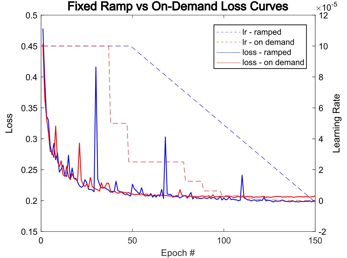
Fig 1: A plot of loss curves with its applied learning rate curves as training progresses with each epoch. The left side axis measures the loss value, and the right side axis describes the value of the learning rate. The red lines correspond to a run with an on-demand learning rate policy and the blue lines correspond to a ramped learning rate policy. The two runs were conducted with 576 time steps and training data obtained from normal subjects only.
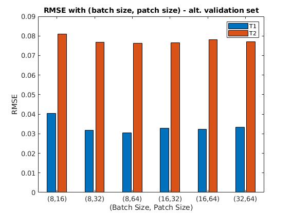
Fig 2: This plot shows the mean RMSE scores of our testing set through training with different pairs of (batch size, patch size). These tests were conducted with 432 time steps and only volunteer data. The lowest T1, T2 score pairing was observed at (8,64), with RMSE = 0.031, 0.076 respectively.
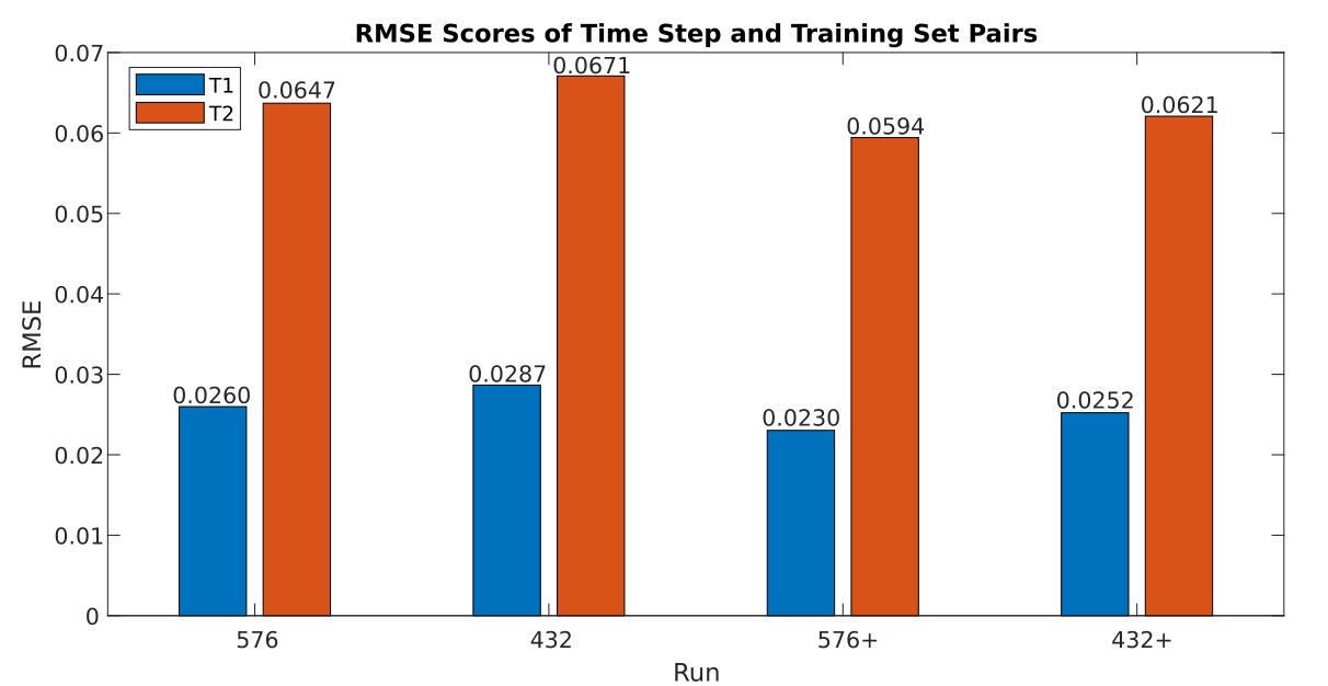
Fig 3: This plot depicts the average RMSE scores of different tests with only their number of time frames and training set varied. Results marked with ‘576’ and ‘576+’ both were trained with 576 time steps, and “+” indicates that patient data has been added to the original training set of only normal subject scans. Results marked with ‘432’ and ‘432+’ both were trained with 432 time frames and “+” is used here likewise. The addition of patient scans increased performance slightly from their normal-subject-only counterparts and the lowest RMSE scoring pair was observed for the case of ‘576+’.
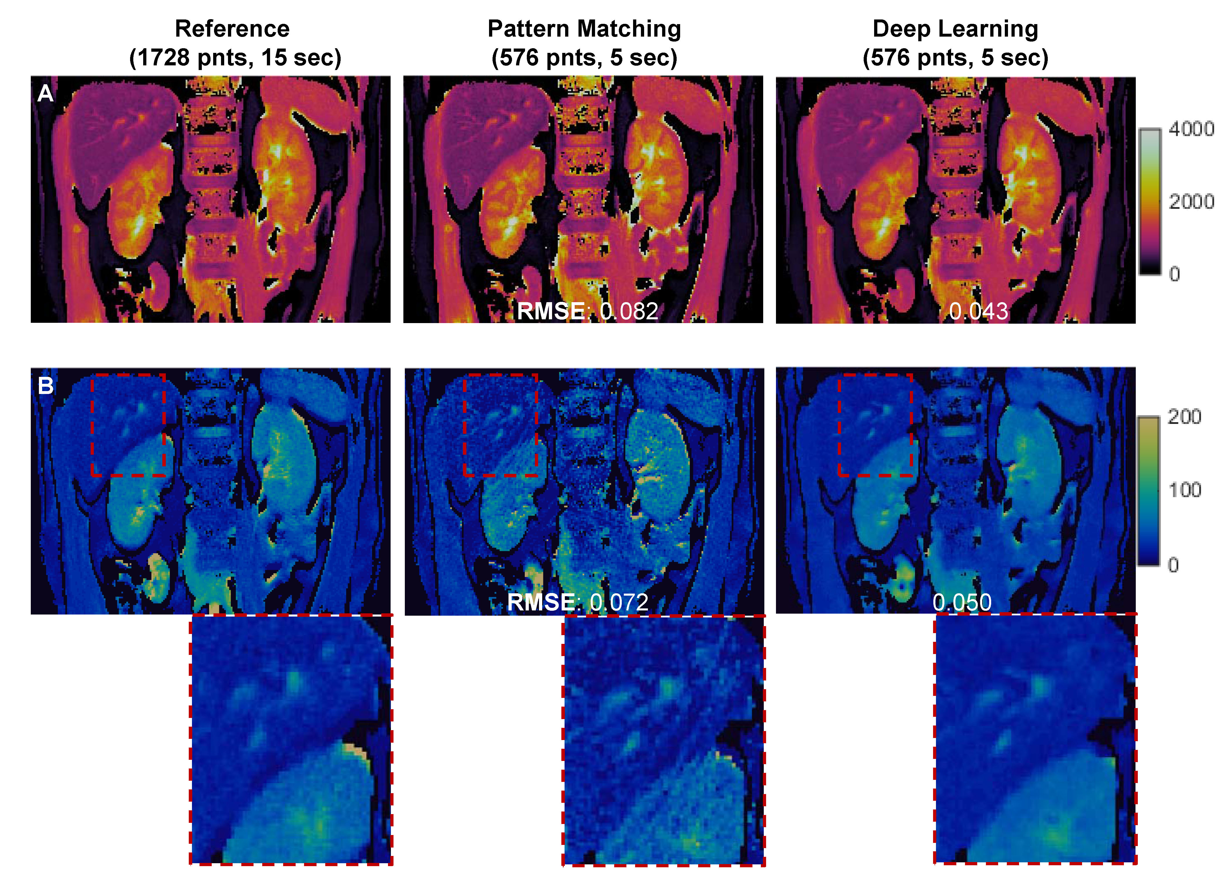
Fig 4: Comparison of T1 (A) and T2 (B) maps obtained using dictionary pattern matching and deep learning. Both results were obtained using 33% of total time points, corresponding to 5-sec scan time. The pattern matching results obtained using all 1728 points (15 sec) were used as the reference to calculate RMSE values.
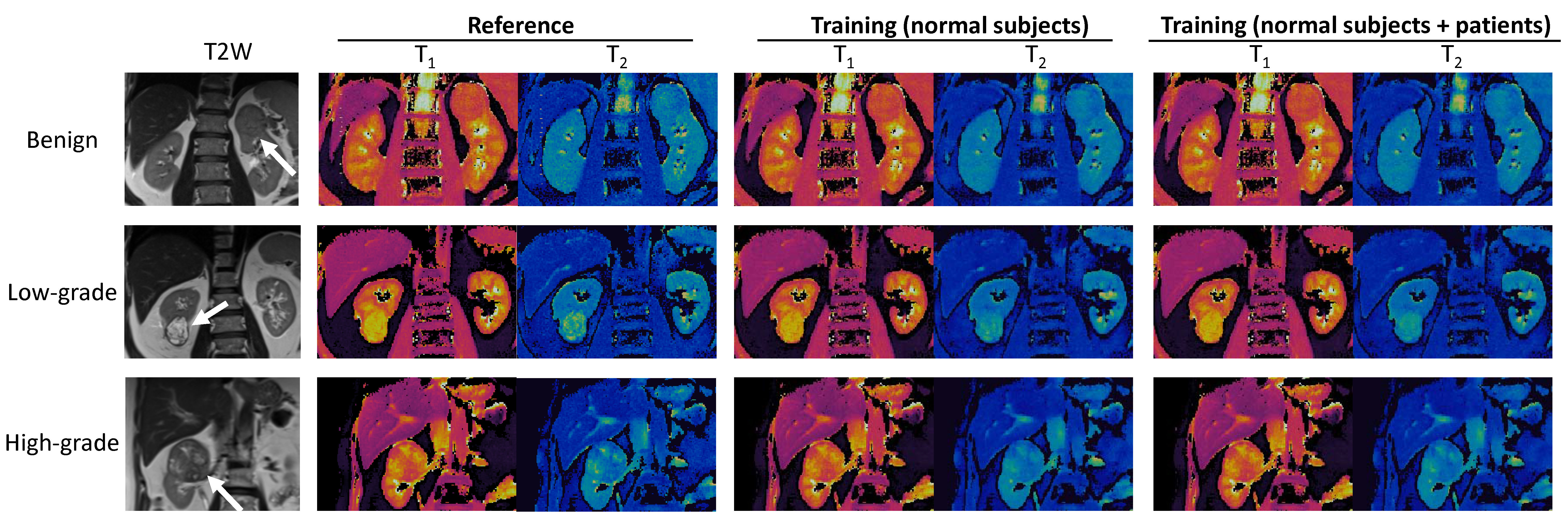
Fig 5: MRF T1 and T2 maps obtained from three patients with benign, low-grade and high-grade renal cell carcinoma. The reference maps (left column) were obtained using pattern matching and all 1728 time frames, while the deep learning results (right two columns) were obtained using only one third of the time points. Results obtained from two training datasets, with and without patient scans, are both presented.
DOI: https://doi.org/10.58530/2023/3631