Synopsis

Keywords: Software Tools, Diffusion Tensor Imaging, Low-field

A super-resolution approach was used to create 2mm isotropic diffusion tensor images (DTI) from diffusion-weighted imaging data acquired on a low field, portable system. Mean diffusivity, fractional anisotropy and principal eigenvector orientation maps are shown. This work extends the very recently implemented capability of performing DTI on a 64mT system, and shows substantial improvement due to the increased through-plane resolution achieved with super-resolution.

Introduction

Low-cost, low-field MRI systems can increase accessibility to MRI in locations where higher-field systems are unavailable. Functionality of a 64 mT, portable MR system (Swoop, Hyperfine Inc., Guilford, CT) was recently extended to perform diffusion-weighted imaging (DWI)¹ and diffusion tensor imaging (DTI)², both of which can provide valuable, non-invasive insight into clinically- and developmentally-relevant metrics (e.g., refs 3-5). Nevertheless, the low signal-to-noise ratio available at 64 mT means that image resolution in the slice direction is generally poor (~6mm in ref. 2). Here, we employ a super-resolution approach based on ref [6] to reconstruct 2mm isotropic DTIs from DWIs acquired at 64 mT.

Methods

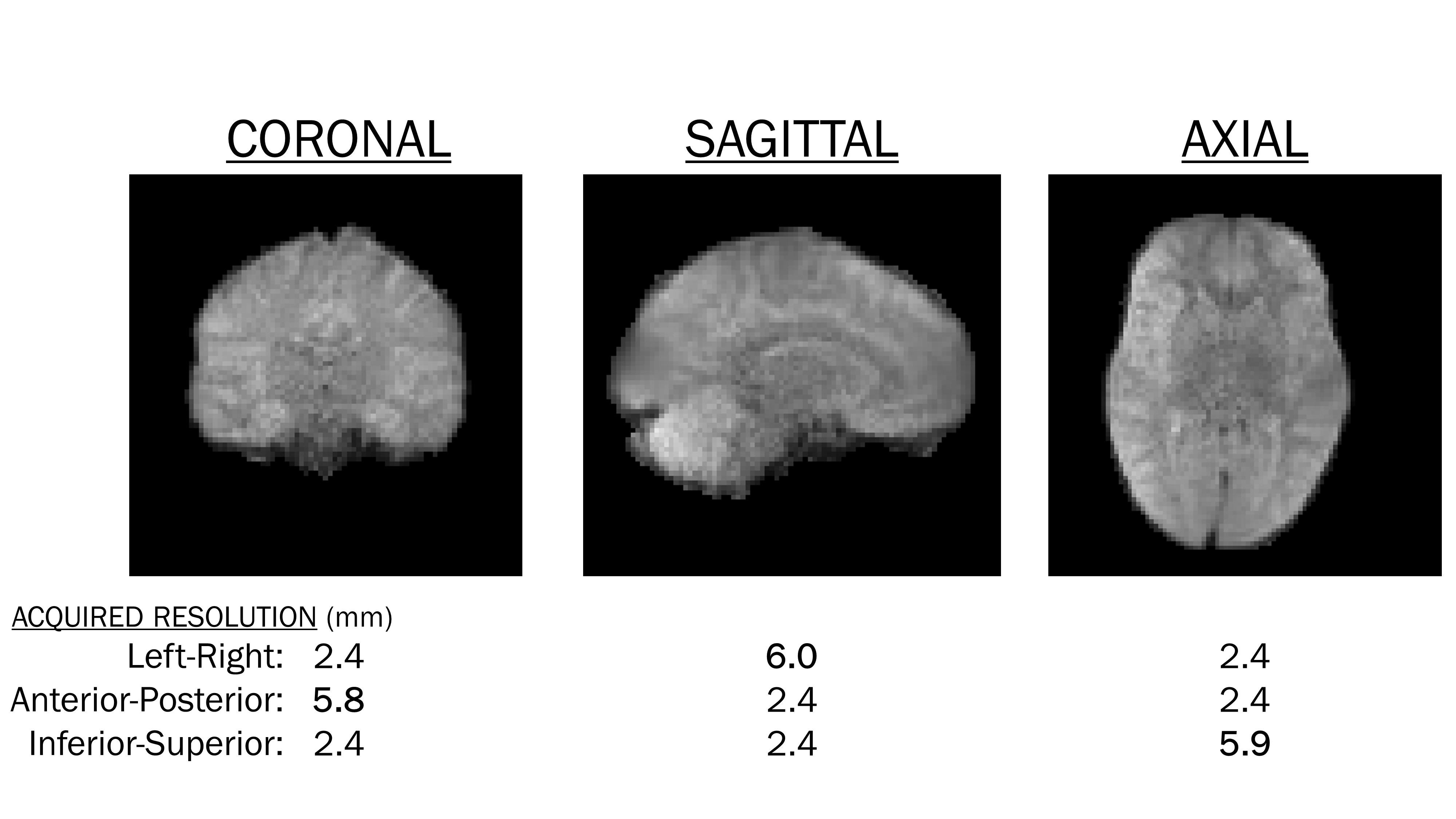
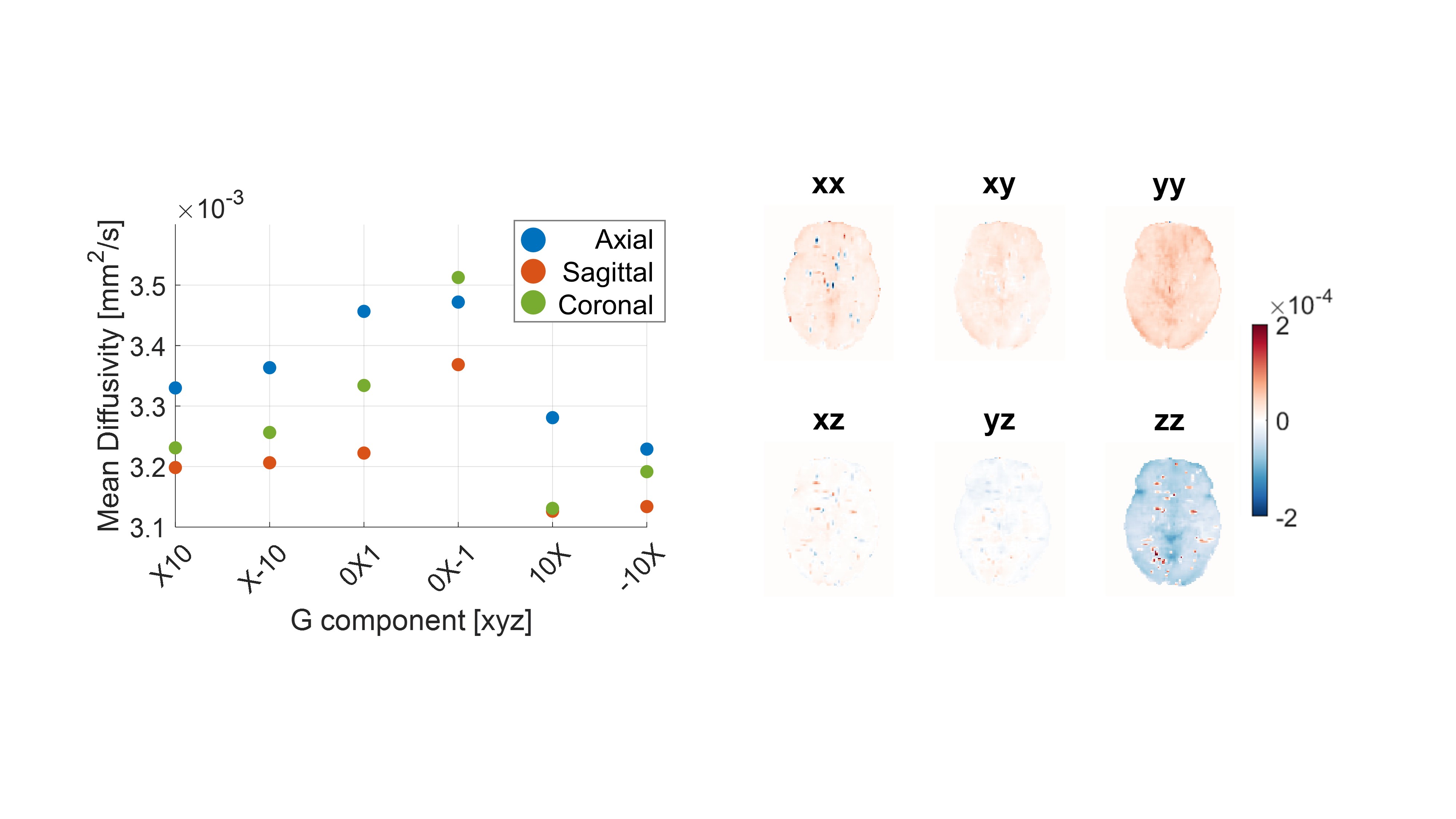
Data was acquired on a Hyperfine Swoop (hardware version 1.7, software version 8.5). A six-direction optimised icosahedral scheme⁷ was used to acquire DWIs at b=600 s/mm², along with a b=0 s/mm² image. Two averages were acquired for each direction using a 3D turbo spin echo sequence with navigator echo, hysteresis correction and eddy current pre-compensation as described in¹. The six DWI (and b=0 s/mm²) scans were repeated for three orthogonal acquisitions (a total of 18 DWI volumes), varying the low-resolution through-plane direction, which was inferior-superior, anterior-posterior, and left-right for axial, coronal and sagittal acquisitions, respectively (figure 1). TE and TR were 86ms and 1s, respectively. Total scan time was approximately 90 minutes.

Data were de-noised using block-matching and 4-D filtering⁸ and brain extraction was performed using FSL’s bet⁹. The axial, coronal and sagittal b=0 s/mm² images were combined to form one 2mm isotropic image using ANTs’ antsMultivariateTemplateConstruction2 tool¹⁰. The affine and warp transformations applied to each b=0s/mm² image were saved. Next, the following steps were applied independently to the axially-, coronally- and sagittally-acquired DWI data:

1) The diffusion tensor was fit with least squares estimation using FSL’s dtifit, and the six unique tensor elements were extracted.
2) The corresponding previously-saved transformations were applied to each tensor element using antsApplyTransforms.
3) The effect of the transformations on the diffusion tensor was corrected using ANTs ReorientTensorImage.

Finally, the three DTIs were averaged using ANTs AverageTensorImage, yielding a 2mm isotropic DTI. Mean diffusivity, fractional anisotropy and RGB (principal eigenvector) maps were generated using ANTs ImageMath functions.

Results and Discussion

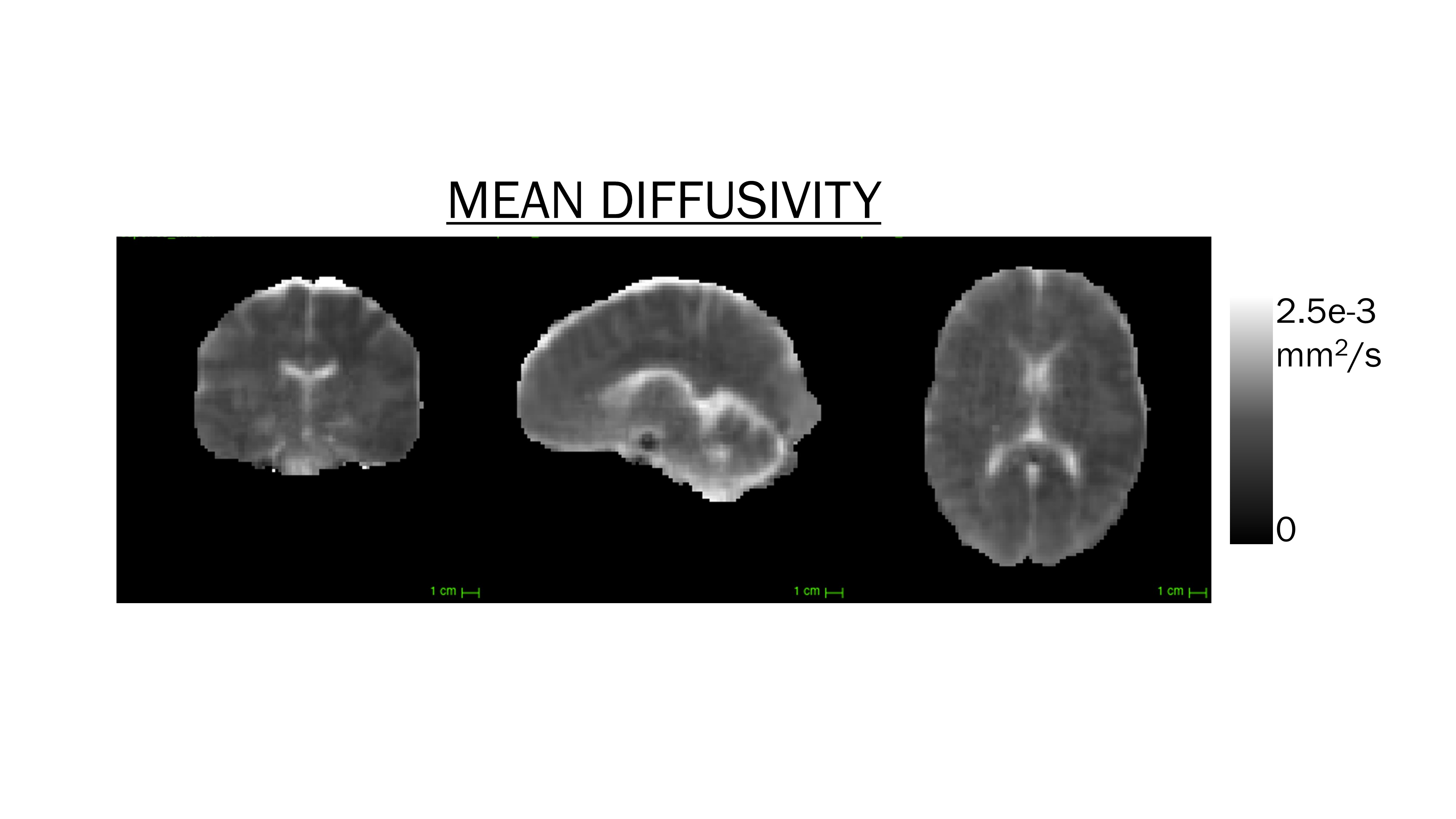
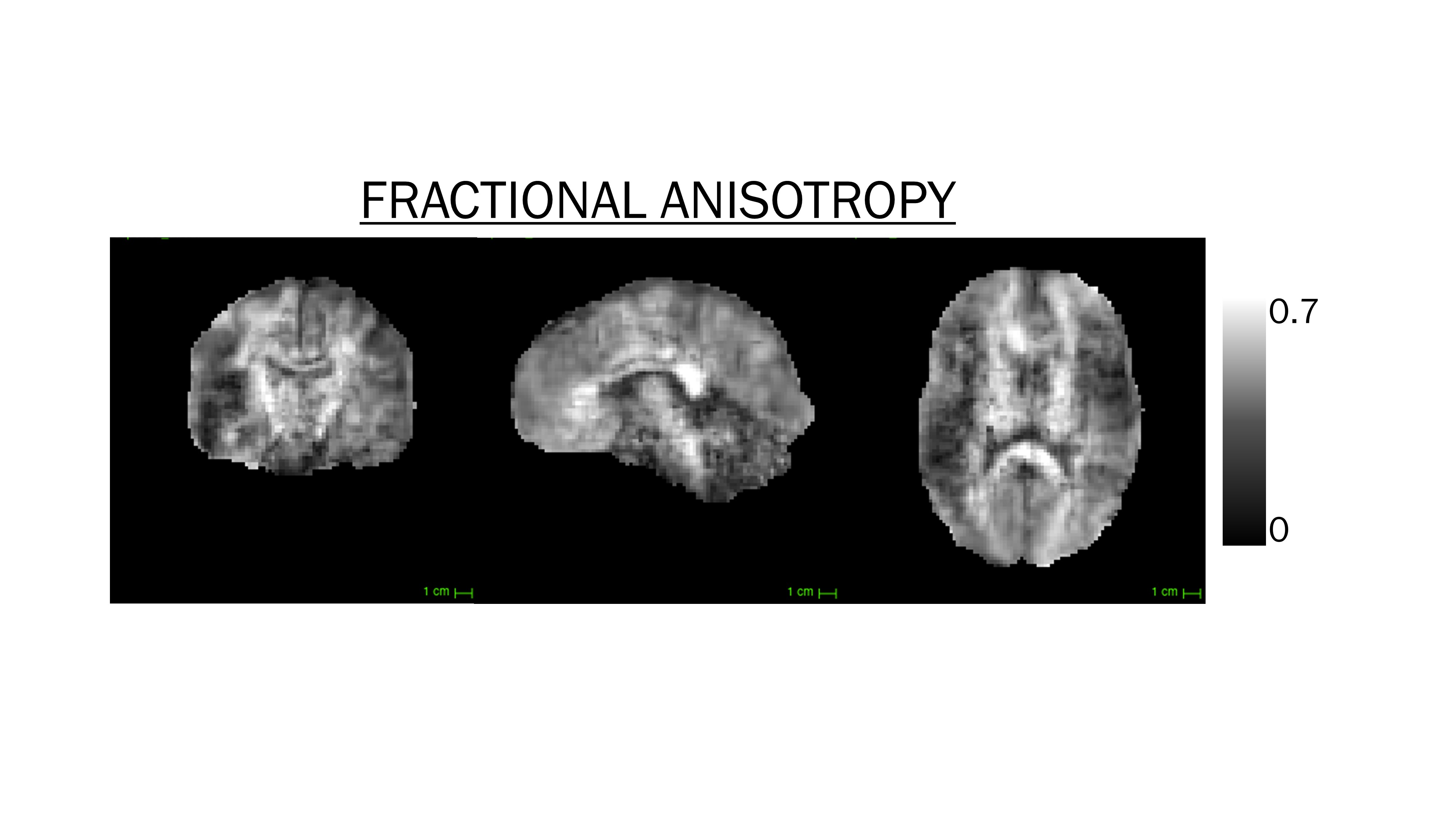
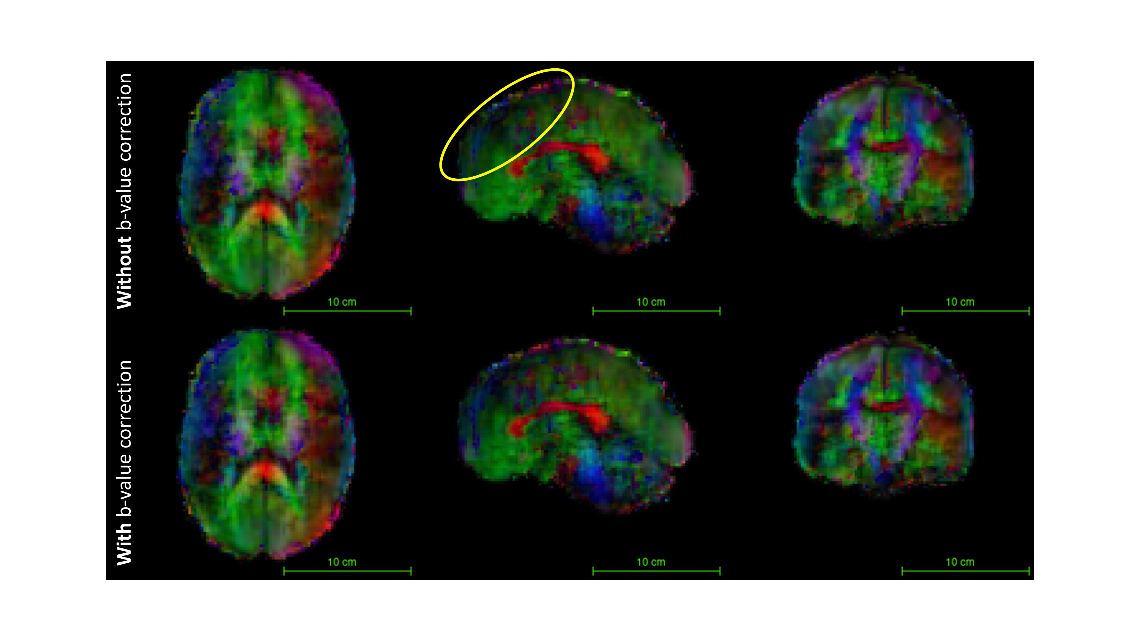
Figure 2 shows mean diffusivity (MD) values. White matter, grey matter and cerebrospinal fluid (CSF) showed good contrast, and were in line with known MD values (e.g., ~.0022 mm²/s in CSF¹¹). Fractional anisotropy (FA) maps are shown in figure 3. The super-resolved volume clearly delineates the major white matter tracts in all three viewing planes.

Red-green-blue (RGB) fibre orientation maps are shown in figure 4. Although the major tracts were clearly visible in all three viewing planes, the principal eigenvector revealed a bias in the anterior-posterior direction (apparent from the dominance of green colour in figure 4a). This was also apparent when looking at the diffusion tensor elements, where the Dyy component was substantially stronger than the other elements (data not shown). We therefore applied a correction by modifying the b-value used in the initial tensor calculation. Specifically, MD was measured in a water phantom using the same six-direction, three-plane scheme. The overall average MD value was used to establish a relative scaling factor for each gradient direction and each acquisition plane, which was subsequently applied to the in-vivo data. The correction yielded a reduction in the Dyy component (and an increase in the Dzz component), as anticipated (figure 5b).

Resultant modest but appreciable improvements to the principal eigenvector were present (figure 4b), most clearly noticeable in the anterior part of the brain (yellow circle), where the anterior-posterior components (green) were somewhat reduced. The calibration (phantom) data used to calculate the correction factor contained only four averages. We believe that further improvements could be made by increasing the number of averages in this data. The benefits of the increased through-plane resolution offered by the super-resolution approach are clear – compared to ref 2, the coronal and sagittal viewing planes offer rich and detailed structural information; the coherence of which are otherwise compromised with large voxels in the through-plane dimension. Future directions include incorporating machine learning approaches to reduce the acquisition time - the most restricting factor for clinical practice.

Conclusion

Diffusion tensor MR-imaging was performed on data acquired from a 64 mT portable system. A super-resolution technique was applied to combine diffusion-weighted images acquired in three orthogonal imaging planes, resulting in 2mm isotropic resolution. Mean diffusivity, fractional anisotropy and principal eigenvector maps show detailed white-matter structure for major tracts as well as good grey-white matter contrast in the three viewing planes.

Acknowledgements

This work was made possible by generous support from the Bill and Melinda Gates Foundation through the award of the UNITY project, and through the Wellcome LEAP 1kD programme. ÁP-G was supported by the European Union (NextGenerationEU).