Synopsis

Keywords: Machine Learning/Artificial Intelligence, Diffusion Tensor Imaging

One shortcoming of diffusion MRI (dMRI) is long scan times as numerous images have to be acquired to achieve a reliable angular resolution of diffusion gradient directions. In this work we introduce gauge equivariant convolutional neural network (gCNN) layers that overcome the challenges associated with the dMRI signal being acquired on a sphere instead of a rectangular grid. We apply this method to upsample angular resolution to predict diffusion tensor imaging (DTI) parameters from just six diffusion gradient directions. Additionally, gCNNs are able to train with fewer subjects and are general enough to be applied to other dMRI related problems.

Introduction

Diffusion MRI (dMRI) is a powerful technique for non-invasive mapping of tissue microstructure. One drawback of dMRI is that it requires multiple images for a high angular resolution to reliably estimate model parameters, leading to longer scan times. One approach to shorten scan times is by convolutional neural networks(CNNs) to estimate dMRI parameters acquired with fewer images. Conventional CNNs focus on images, i.e, data on a flat euclidean manifold, however, dMRI is acquired on a sphere, which is a non-euclidean manifold. One elegant way to construct CNNs on non-euclidean manifolds is to use gauge-equivariant CNNs (gCNNs)¹. Gauge-equivariant networks use group theory to perform generalized convolutions on arbitrary geometries, and are efficient because of their invariance to rotation, and implementations built using 2D convolution layers. These networks have shown promise in computer vision applications, but have yet to be applied to dMRI. Architectures built with gCNN layers are able to take advantage of the symmetry inherent in diffusion data, require fewer samples for training, and are general enough to be applied to a wide range of problems. In this work we introduce the theory and an initial architecture to perform DTI denoising from dMRI acquisitions with only six directions.

Methods

In DTI the signal is modeled with the following equation,
$$S_k\left(\vec{x}\right) = S_0 e^{ -b \vec{g}_k^T D(\vec{x}) \vec{g}_k },$$ (1)
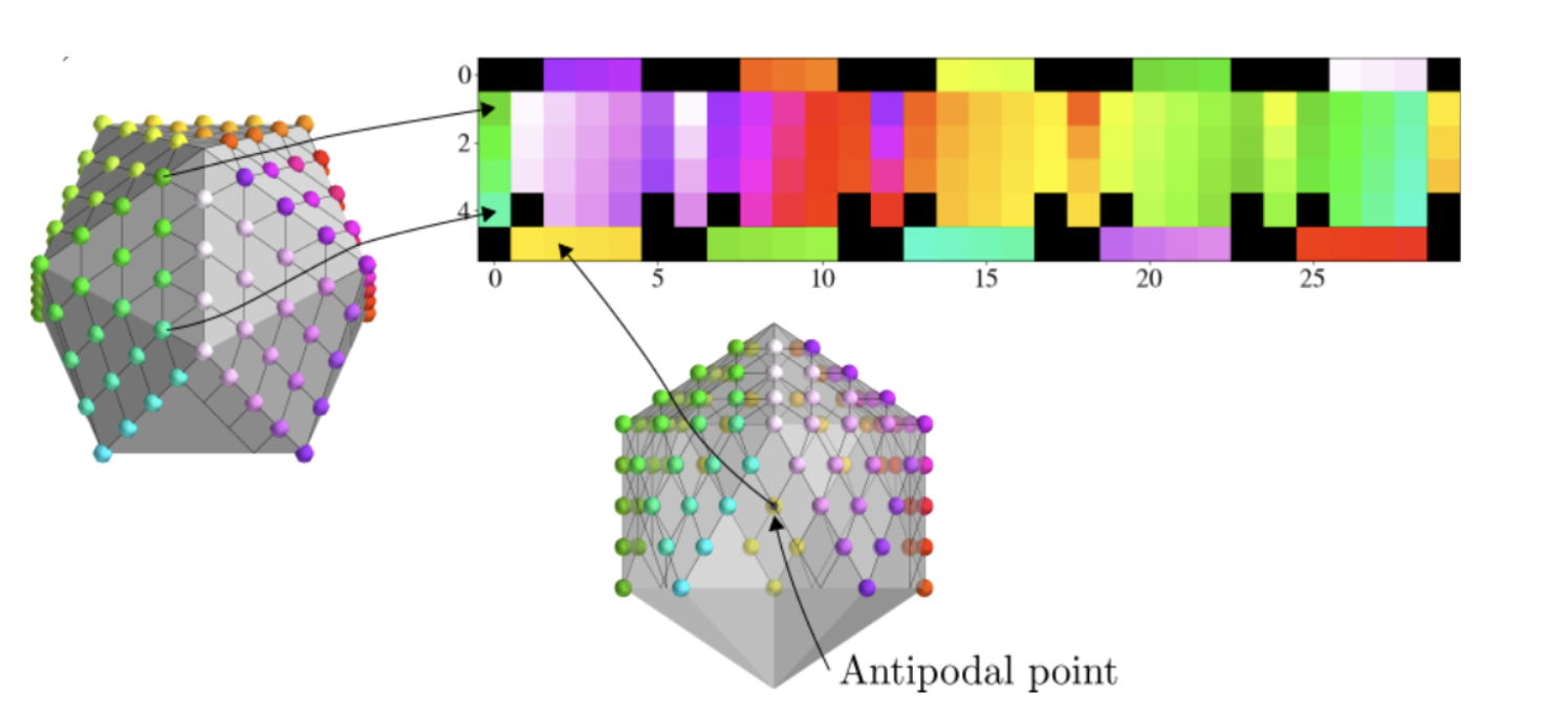
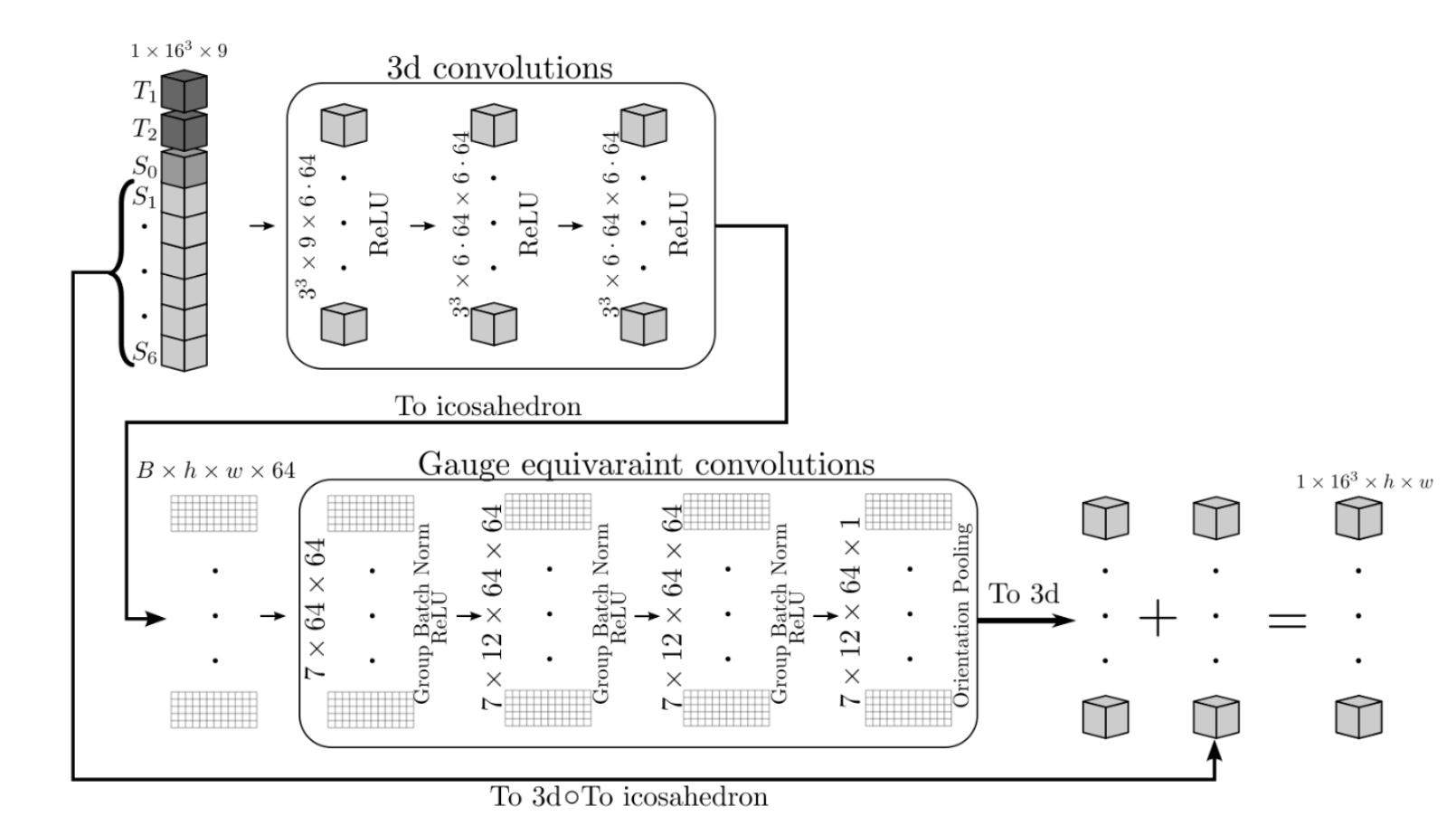
where $$$S_0$$$ is a constant, $$$D(\vec{x})$$$ is the diffusion tensor field, $$$\vec{g}_k$$$ is a unit vector, and $$$b$$$ is the b-value. A typical dMRI acquisition will have many images, $$$k \in \{1, ..., N_\text{directions}\}$$$, such that the unit vectors $$$\vec{g}_k$$$ are spread evenly over a sphere. We see from (1) that $$$S_k$$$ has antipodal symmetry, i.e., it is invariant under the transformation $$$\vec{g}_k \rightarrow -\vec{g}_k $$$. Hence, we assume that the signal is a function of all unoriented lines from the origin of $$$\mathbb{R}^3$$$, i.e., the real projective plane, $$$\mathbb{R}P^2$$$. A model of $$$\mathbb{R}P^2$$$ can be constructed by a sphere with antipodal points identified and then extracting the top hemisphere which can then be flattened in a manner similar to the treatment in Cohen et al.1 , as illustrated in Fig 1. Note that when comparing to the work of Cohen et al.¹, which uses a full sphere, we use the full dihedral group that includes reflections and rotations of the hexagonal filters. We implemented gauge-equivariant layers for the half-sphere in PyTorch, and provide an open-source package, gcnn-dmri (http://github.com/khanlab/gcnn_dmri), to incorporate these layers into novel architectures . As an initial demonstration, we implemented a network to perform DTI denoising, using an approach inspired by the residual network used in DeepDTI². The input of the network is $$$16\times16\times16$$$ blocks of $$$T_1$$$,$$$T_2$$$, $$$S_0$$$, and six images $$$S_1, ..., S_6$$$ corresponding to the six gradient directions with b-value $$$1000 \text{s}/\text{mm}^2$$$. The directions are simply taken to be the first six in the acquisition, which is done to mimic an early stop of the scan session. A mean squared error loss is used to compare the network output with the DTI signal as generated from 90 directions with a b-value of $$$1000 \text{s}/\text{mm}^2$$$. Fig 2 shows the architecture. After training, DTI metrics are computed from the predicted signal using FSL’s³ dtifit https://fsl.fmrib.ox.ac.uk/. We used the available pre-processed dMRI data from the Human Connectome Project (HCP) Young Adult 3T study⁴, with 15 random subjects for training, and 25 random subjects for testing. Freesurfer5 was used to obtain a foreground mask that excludes the cerebrospinal fluid. Structural T1-weighted and T2-weighted images were resampled to the resolution of the dMRI images. The network was trained for 20 epochs, with a learning rate of $$$1\times10^{-4}$$$ on two V100 GPUs.

Results

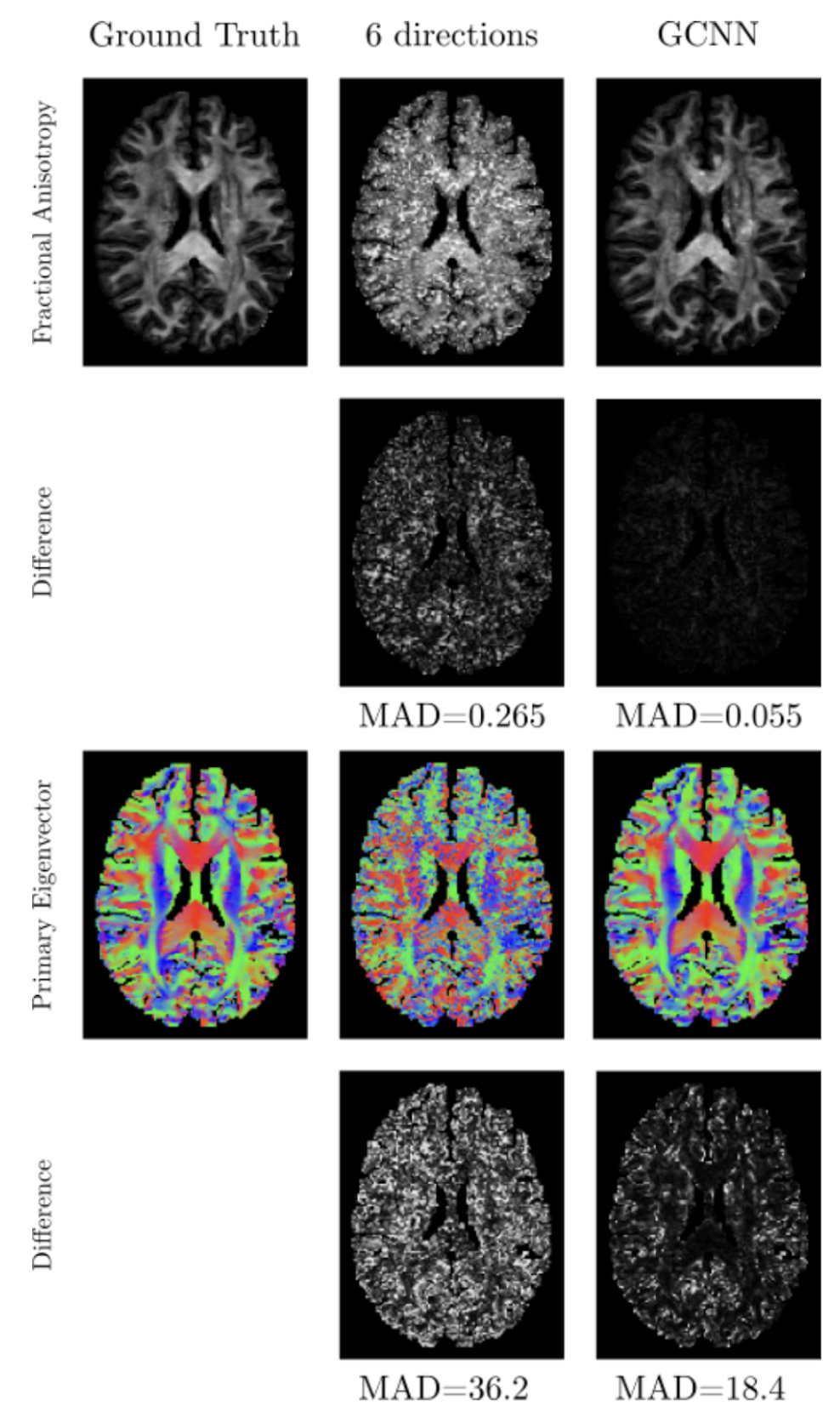
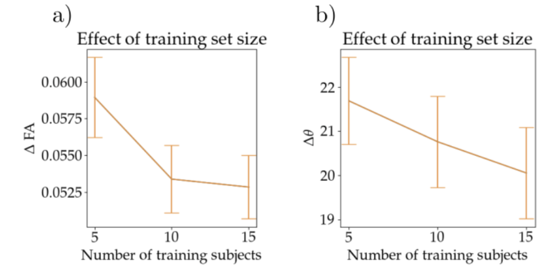
In Fig 3 we show the result of one subject of our network for fractional anisotropy (FA) (first two rows) and the primary eigen vector V1 (last two rows). The left column shows the ground truth parameter using 90 directions, the middle column shows the result for using six directions and the right column shows the result from using gCNNs. Also shown are the mean absolute differences (MAD) between six directions and ground truth, and between the gCNN result and the ground truth. Fig 4 shows the means and standard deviation over 25 test subjects of MAD for FA and V1 for using 5, 10 and 15 subjects for training.

Discussion

Our work shows how gCNNs can be used to mitigate the challenges associated with the non-euclidean geometry (sphere or real projective plane) of the dMRI signal. In this work we introduce gCNNs layers and apply it to the problem of denoising DTI parameters from acquisitions with low angular resolution. Our work is similar to that of Tian et al.² where they are able to reach a reduction in MAD of 34% for FA and about 53% for V1 (from Fig. 5 in Tian e. al.²) which is consistent with our results at 21% for FA and 50% for V1, but with the advantage of using significantly fewer training subjects (15 compared 40) and the freedom of using any six directions. In addition, these gCNNs layers are general and can be used for other dMRI related problems like kurtosis, tractography, data harmonization etc.

Acknowledgements

During the course of this work UH was supported by a postdoctoral fellowship from the Canadian Open Neuroscience Platform (CONP). AK was supported by the Canada Research Chairs program #950-231964, NSERC Discovery Grant #6639, and Canada Foundation for Innovation (CFI) John R. Evans Leaders Fund project #37427, the Canada First Research Excellence Fund, and Brain Canada.