3575
Realistic Abdominal QSM phantom1Department of Electrical Engineering, Pontificia Universidad Catolica de Chile, Santiago, Chile, 2Biomedical Imaging Center, Pontificia Universidad Catolica de Chile, Santiago, Chile, 3Millennium Institute for Intelligent Healthcare Engineering (iHEALTH), Santiago, Chile, 4School of Electrical Engineering, Pontificia Universidad Catolica de Valparaiso, Valparaiso, Chile, 5Department of Radiology, Pontificia Universidad Catolica de Chile, Santiago, Chile
Synopsis
Keywords: Signal Modeling, Susceptibility
Abdominal Quantitative Susceptibility Mapping (QSM) involves a series of additional challenges compared with brain QSM, mainly because of the presence of undesired contributions related to fat and gasses. Previously, we proposed a QSM phantom with fat contributions, which emulated different susceptibility scenarios in the abdominal region. In this work, we present an improved version which now considers additional features including a variable multi-peak fat model, variable R2* and background field features. Simulation experiments show how these new components produce of different effects, like increased signal decay in specific tissues, 1st and 2nd kind chemical shift artifacts and water/fat swaps in graph cuts reconstructions.Introduction
Quantitative Susceptibility Mapping [1] has gained interest for applications outside the brain, especially as a biomarker for iron overload [2,3] and fibrosis [4,5] in the abdominal region. However, the presence of fat, gastrointestinal gasses, and different kinds of motion results in a more challenging problem, with different acquisition restrictions and additional preprocessing steps [6,7]. For brain applications, reconstruction strategies are evaluated using in-vivo ground truths [8] and experimental or in-silico phantoms [9,10]. Nevertheless, for the abdomen these approaches suffer from several limitations: it is not possible to acquire in vivo ground truths via multiple orientations, the experimental phantoms consist of vials and bottles with unrealistic geometries [11], and in-silico phantoms typically consist of mesh models with piecewise values [12,13]. To address this problem, we previously proposed a realistic QSM phantom of the abdomen with fat contributions and modifiable susceptibility values [14]. However, the scope of that work was limited to susceptibility scenarios, with static values for the rest of the tissue properties. In order to achieve simulations closer to experimental acquisitions effects, we included new features: a modifiable R2* map for signal decay, multiple peak models for the fat spectrum, corrected and non-corrected background field contrubutions and the possibility to simulate 1st and 2nd kind chemical shift artifacts.Methods
R2* model:We used a similar heuristic as that proposed for our previous model [14], but texture parameters related to water and fat were neglected. Thus, in order to modify a tissue class selected by setting the binary variable to 1, is given by:
$$R_{2,t}^{\ast,s}=\begin{cases}R_{2}^{*}\left(r\right) & \text{if }m_{t}=0\\\overline{R_{2,t}^{}}+a_{t}\cdot\left(r_{2}^{}\left(r\right)-\overline{r_{2,t}^{*}}\right) & \text{if }m_{t}=1\end{cases}$$
where $$$R_{2,t}^{\ast,s}$$$ is the synthetic $$$R_{2}^{*}$$$ value of the tissue class $$$t$$$ at the voxel $$$r$$$ , $$$R_{2}^{*}(r)$$$ is an experimental $$$R_{2}^{*}$$$ map, $$$\overline{R_{2,t}^{\ast}}$$$ is the mean $$$R_{2}^{*}$$$ value assigned to the tissue class $$$t$$$, $$$r_{2}^{*}$$$ is the experimental $$$R_{2}^{*}$$$ normalized to the 0 to 1 range and $$$\overline{r_{2,t}^{\ast}}$$$ is its mean value for the whole tissue class $$$t$$$. The value of the $$$a_{t}$$$ parameter was chosen so that the resulting synthetic map acquired a realistic non-smooth texture.
Background fields:
For local synthetic susceptibility $$$\chi_{\text{local}}^{s}$$$ , all tissues excluding the air regions were considered inside the region of interest. External and gastrointestinal air susceptibility values were set as 9.2 [9] and 4.84 [15], respectively and were considered as the only tissues outside the region of interest, as part of the background susceptibility $$$\chi_{\text{background}}^{s}$$$ . Then, total field was computed as a point-wise multiplication of the sum of both components with the dipole kernel $$$D(r)$$$ in the Fourier domain [16].
$$\delta_{\chi}\left(r\right)=\mathcal{F}^{-1}\left[\mathcal{F}\left(\chi_{\text{local}}^{s}\left(r\right)+\chi_{\text{background}}^{s}\left(r\right)\right)\cdot\mathcal{F}\left(D\left(r\right)\right)\right]$$
1st kind chemical shift artifacts:
Chemical shift artifacts of the 1st kind were simulated by shifting the fat image $$$\rho_{F}(r)$$$ in $$$\frac{f_{m}\cdot B_{0}\cdot\gamma}{rBW}$$$ pixels from the k-space, according to
$$\rho_{F}^{\text{shift}}\left(r\right)=\mathcal{F}^{-1}\left[\mathcal{F}\left(\rho_{F}\left(r\right)\right)\cdot\sum_{m=1}^{N}a_{m}\cdot e^{-i\cdot2\pi\cdot\frac{f_{m}\cdot B_{0}\cdot\gamma}{rBW}\cdot k_{x}}\right]$$
were $$$f_m$$$ and $$$\alpha_m$$$ are the relative frequencies and amplitudes of the selected fat model, $$$B_0$$$ is the fieldmap strength of 3 T, $$$\gamma$$$ is the gyromagnetic ratio and $$$rBW$$$ is the receiver bandwidth in Hz/pixel.
Multipeak fat models:
Multipeak fat models were included by modifying our signal model [14] to:
$$S\left(r,TE_{k}\right)=\left(\rho_{W}\left(r\right)+\rho_{F}^{\text{shift}}\left(r\right)\cdot\sum_{m=1}^{N}a_{m}\cdot e^{\cdot2\pi\cdot B_{0}\cdot\gamma\cdot f_{m}\cdot TE_{k}}\right)\cdot e^{\left[-R_{2}^{*,s}\left(r\right)+i\cdot2\pi\cdot B_{0}\cdot\gamma\cdot\delta_{\chi}\left(r\right)\right]\cdot TE_{k}}$$
Were $$$ S\left(r,TE_{k}\right) $$$ is the simulated signal for the voxel $$$r$$$ at the $$$k$$$-th echo time $$$TE_k$$$ and $$$\rho_W$$$ is the water image.
Results
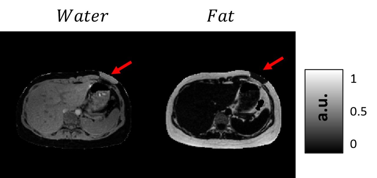
Figure 1 shows the generation of different tissue properties for different scenarios. It can be seen how the R2* maps are continuous and generate an abrupt decay in the last echo times. Figure 2 shows the simulation of chemical shift artifacts of the 1st kind for 4 different receiver bandwidths. It can be seen than there is no significant difference between the shifts for 1, 6 and 9 peaks models. Figure 3 shows the magnitude images for 3 different acquisition protocols, consistent in a chemical shift encoded protocol, and two 1-peak-based in-phase protocols for 2 different fat models. It can be seen how the first and third protocols present out-phase artifacts due to the echo time mismatch with the 6 peak fat model. Figure 4 shows local and total fieldmap reconstruction for two different approaches. While the in-phase reconstructions with ROMEO present well estimated local and total fieldmap, iterative graph cuts fails at estimating the total fieldmap, resulting in water-fat swap artifacts, which can be seen in the Figure 5.Discussion & Conclussion
We created a realistic in silico phantom for abdominal QSM with a set of different tissue properties. The phantom simulates different acquisition and reconstruction artifacts associated with chemical shift and background removal, which could be a valuable tool for assessing QSM reconstruction algorithms in the abdominal region.Acknowledgements
This work has been funded by the following grants: Fondecyt 1191710 and 1231535, Anillo ACT912064, Millennium Institute for Intelligent Healthcare Engineering, iHEALTH (ICN2021_004).References
1. Wang Y, Liu T. Quantitative Susceptibility Mapping (QSM): Decoding MRI Data for a Tissue Magnetic Biomarker. Magnetic Resonance in Medicine 2014; 73:82–101.
2. Sharma SD, Hernando D, Horng DE, Reeder SB. Quantitative susceptibility mapping in the abdomen as an imaging biomarker of hepatic iron overload. Magn Reson Med 2015; 74:673–683
3. Sharma SD, Fischer R, Schoennagel BP, Nielsen P, Kooijman H, Yamamura J, Adam G, Bannas P, Hernando D, Reeder SB. MRI-based quantitative susceptibility mapping (QSM) and R2* mapping of liver iron overload: Comparison with SQUID-based biomagnetic liver susceptometry. Magn Reson Med. 2017;78(1):264-270
4. Jafari R, Hectors SJ, Koehne de González AK, Spincemaille P, Prince MR, Brittenham GM, Wang Y. Integrated quantitative susceptibility and R2 * mapping for evaluation of liver fibrosis: An ex vivo feasibility study. NMR Biomed. 2021;34(1):e4412
5. Bechler, E., Stabinska, J., Thiel, T., Jasse, J., Zukovs, R., Valentin, B., Wittsack, H.-J., Ljimani, A., 2021. Feasibility of quantitative susceptibility mapping (QSM) of the human kidney. Magnetic Resonance Materials in Physics, Biology and Medicine 34, 389–397
6. Karsa A, Shmueli K. SEGUE: A Speedy rEgion-Growing Algorithm for Unwrapping Estimated Phase. IEEE Trans Med Imaging. 2019;38(6):1347-1357
7. Jafari R, Sheth S, Spincemaille P, Nguyen TD, Prince MR, Wen Y, Guo Y, Deh K, Liu Z, Margolis D, Brittenham GM, Kierans AS, Wang Y. Rapid automated liver quantitative susceptibility mapping. J Magn Reson Imaging. 2019;50(3):725-732
8. Liu T, Spincemaille P, de Rochefort L, Kressler B, Wang Y. Calculation of susceptibility through multiple orientation sampling (COSMOS): a method for conditioning the inverse problem from measured magnetic field map to susceptibility source image in MRI. Magn Reson Med 2009; 61: 196– 204.
9. Marques JP, Meineke J, Milovic C, et al. QSM reconstruction challenge 2.0: A realistic in silico head phantom for MRI data simulation and evaluation of susceptibility mapping procedures. Magn Reson Med. 2021;86(1):526-542. 10. Milovic C, Bilgic B, Zhao B, Acosta-Cabronero J, Tejos C. Fast nonlinear susceptibility inversion with variational regularization. Magn Reson Med. 2018;80(2):814-821.
11. Hernando D, Cook RJ, Diamond C, Reeder SB. Magnetic susceptibility as a B 0 field strength independent MRI biomarker of liver iron overload. Magn Reson Med. 2013;70(3):648-656.
12. Boehm C, Meineke J, Weiss K, Makowski MR, Karampinos DC. On the water–fat in-phase assumption for quantitative susceptibility mapping (QSM). In: Proceedings of the 31st Annual Meeting of ISMRM. 2022; 2466.
13. Lo W, Chen Y, Jiang Y, et al. Realistic 4D MRI abdominal phantom for the evaluation and comparison of acquisition and reconstruction techniques. Magn Reson Med. 2019;81(3):1863-1875.
14. Silva J, Milovic C, Lambert M, Montalba C, Arrieta C, Uribe S, Tejos C. Realistic in silico abdominal QSM phantom. In: Proceedings of the 31st Annual Meeting of ISMRM. 2022; 1985.
15. Gimsa, J, Haberland, L. Electric and Magnetic Fields in Cells and Tissues. Encyclopedia of Condensed Matter Physics. Condens Matter Phys. 2005; 6-14.
16. Marques JP, Bowtell R. Application of a Fourier-based method for rapid calculation of field inhomogeneity due to spatial variation of magnetic susceptibility. Concepts Magn Reson Part B Magn Reson Eng. 2005; 25B(1):65-78.
Figures
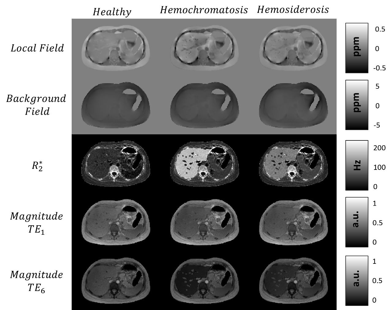
Figure 1:
Tissue properties simulations (local field, background field, R2*) for 3 different cases and magnitude images for first and last echo times.
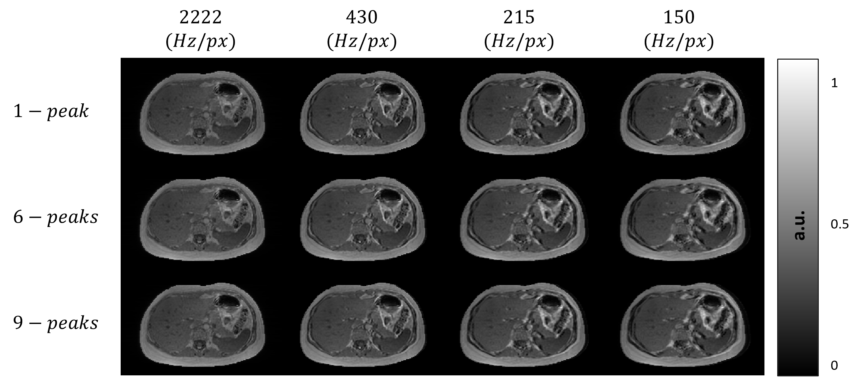
Figure 2:
1st kind chemical shift artifacts simulated for different receiver bandwidths and fat models.
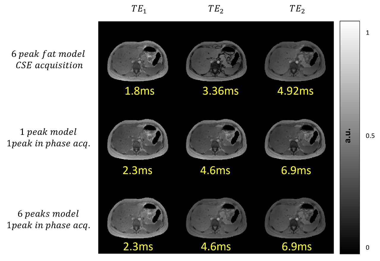
Figure 3:
Magnitudes of first 3 echo times for different simulated acquisition protocols.
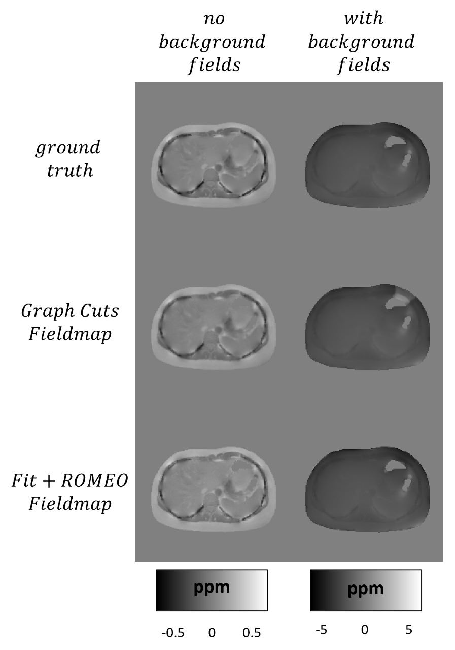
Local and total fieldmap reconstructions.
Example of water/fat swap for Graph Cuts reconstruction.