3573
DeepDECOMPOSE: A Deep Learning based framework for solving DECOMPOSE QSM1Electrical Engineering and Computer Sciences, University of California, Berkeley, Berkeley, CA, United States, 2Helen Wills Neuroscience Institute, University of California, Berkeley, Berkeley, CA, United States
Synopsis
Keywords: Quantitative Imaging, Quantitative Susceptibility mapping
We propose a deep learning (DL) approach to accelerate and improve the accuracy of the parameter fitting problem of DECOMPOSE-QSM. The approach allows a triple complex exponential model to be fitted in <1s on CPUs and <20ms on a GPU for a 256x256 image, vs. 5+ min for the original solver. The DL solver can be implemented with either fixed echo times or adaptive to a range of echo times and number of echoes. Trained with various additive noise levels, the DL-solver performs more robustly compared to the conventional optimization-based solver when the signal has a very low SNR.Introduction
Quantitative susceptibility mapping (QSM) uses a magnetic resonance imaging (MRI) phase contrast to measure the tissue bulk magnetic susceptibility non-invasively[1]. QSM can provide unique contrast in the brain and it has been used in various research fields, such as brain development[2], aging, and neurodegenerative disease studies[3,4,5]. However, with a typical 1 mm resolution, a mixture of bio-molecules with different susceptibility exists within a voxel, causing frequency cancelation resulting in zero QSM values. Models such as DECOMPOSE-QSM[6] and chi-separation[7] are proposed to address this issue with different approaches and considerations. The DECOMPOSE-QSM model solves a nonlinear complex signal model, and calculate paramagnetic component susceptibility (PCS) and diamagnetic component susceptibility (DCS). The DECOMPOSE-QSM model is validated with phantom and ex-vivo temperature-dependent experiments[1]. As the model is highly nonlinear, the long runtime of the optimization-based solver hinders the model from being tested in a large set of cases.Since it is essentially a parameter fitting problem, we developed a multi-layer perceptron (MLP) method trained with synthetic data to estimate of the parameters of the DECOMPOSE model. We show that by training purely on random data [8,9] with temporal additive noise, the deep learning-based solver (DeepDECOMPOSE) is able to achieve the decomposition of QSM and improve robustness to noise.
Methods
[Training strategy]The goal is to perform fast parameter fitting for the DECOMPOSE-QSM[1] model --a summation of three complex exponentials. $$S(t;C_+, C_-, C_0,\chi_+, \chi_-, R_{2,0}^*)=C_+e^{-(a\chi_+ + R_{2,0}^* +i \frac{2}{3}\chi_+ \gamma B_0 )t} + C_-e^{-(a\chi_- + R_{2,0}^* +i \frac{2}{3}\chi_- \gamma B_0 )t} + C_0e^{- R_{2,0}^* t}$$ $$s.t. \ 0< |\chi_{+ or -}| < 0.5 \ \text{and} \ C_+ + C_- + C_0 = 1$$ To start, we generate random values for $$$C_0, C_+, C_-, R_{2,0}^*, \chi_+$$$, and $$$ \chi_-$$$ (with constraints taken into account) that serve as ground truth parameters of the model. The voxel signals are generated using the DECOMPOSE-QSM forward model with specific echo time (TE) arrangements with various levels of noise. DL Solver 1 (S1) with fixed TE is then built to train point-wise on the parameter maps and noisy signal pairs.
Next, to generalize our approach for various numbers of echoes (5-24 are considered), we generate a time grid (0.1ms interval) to fill in the signals based on the TEs. The range of TEs being considered is from 1-51 ms. Essentially, we assign acquired TEs into grids by zeroing out the grid points we do not have, a similar idea to using dropout in a neural network[10]. The inputs are normalized such that they have the same energy with respect to the number of TEs (similar to dropout). We refer to this implementation as adaptive echo Solver 2 (S2).
[Network architecture]
The network structure is shown in Figure 1. The network has five fully connected layers, batch normalization, and hyperbolic tangent as the activation function. While the network solves the inverse problem for each voxel independently, we implemented the network as a fully convolutional neural network (CNN) with 1x1 convolutions to accelerate inference on full images.
Results
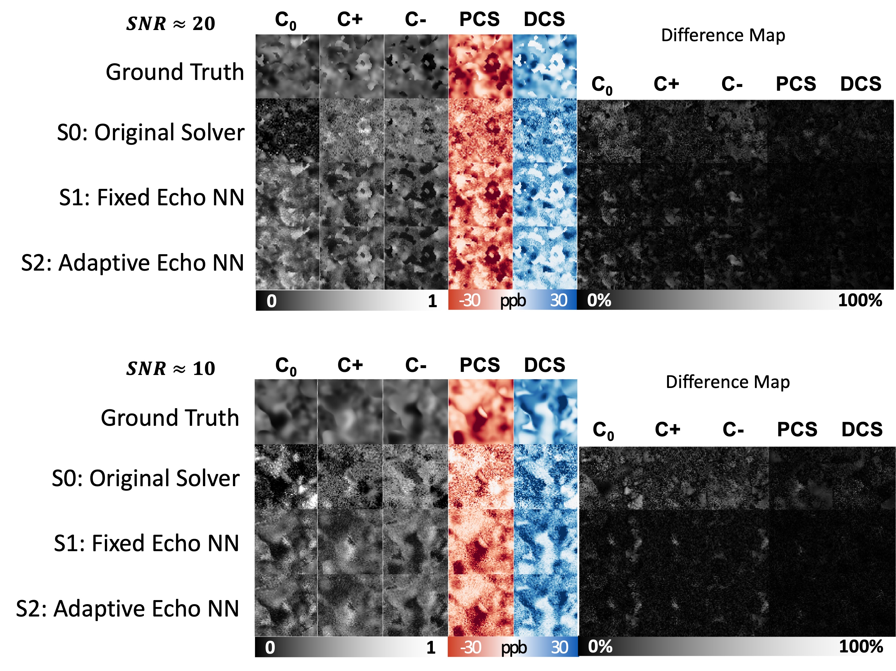
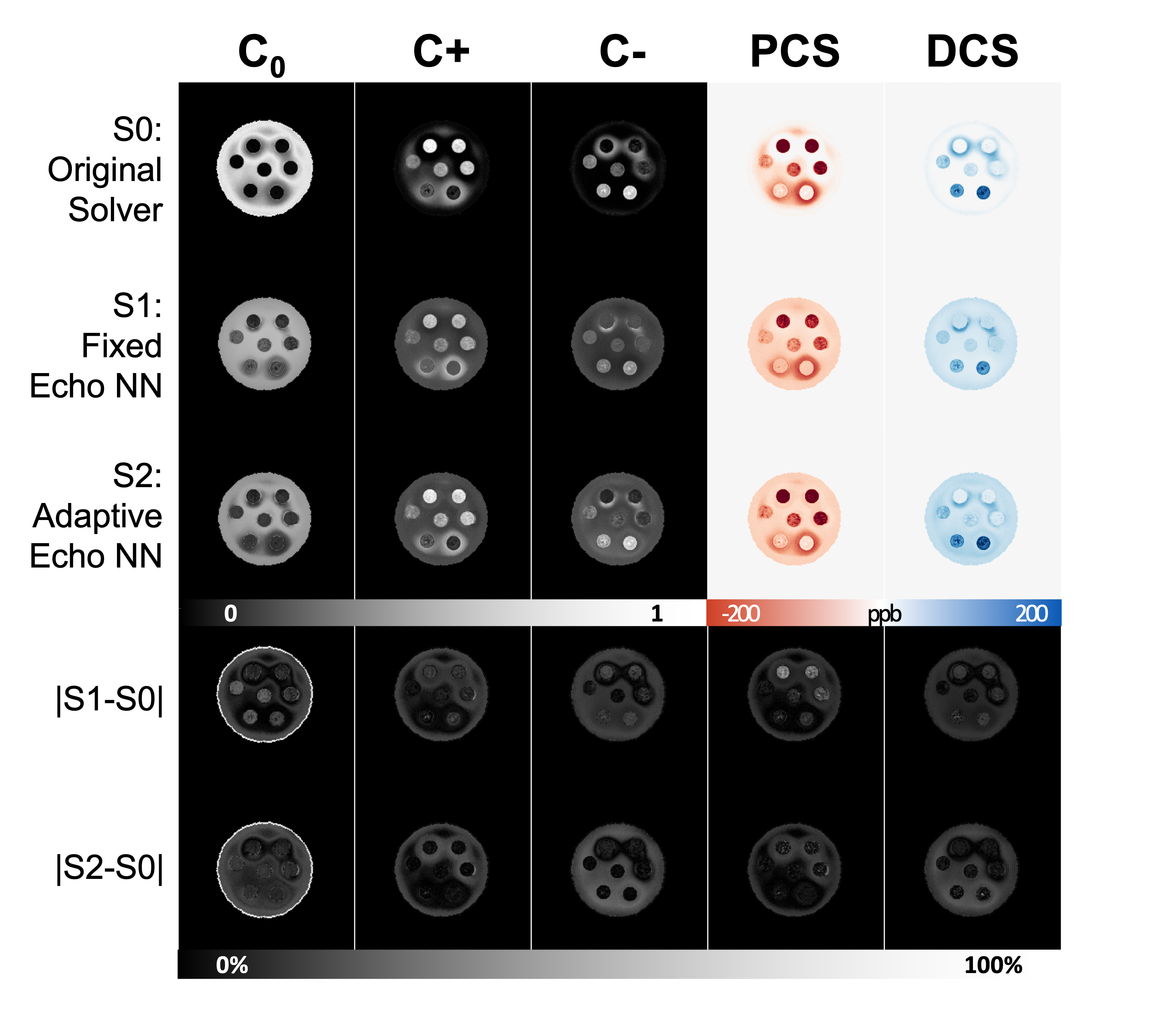
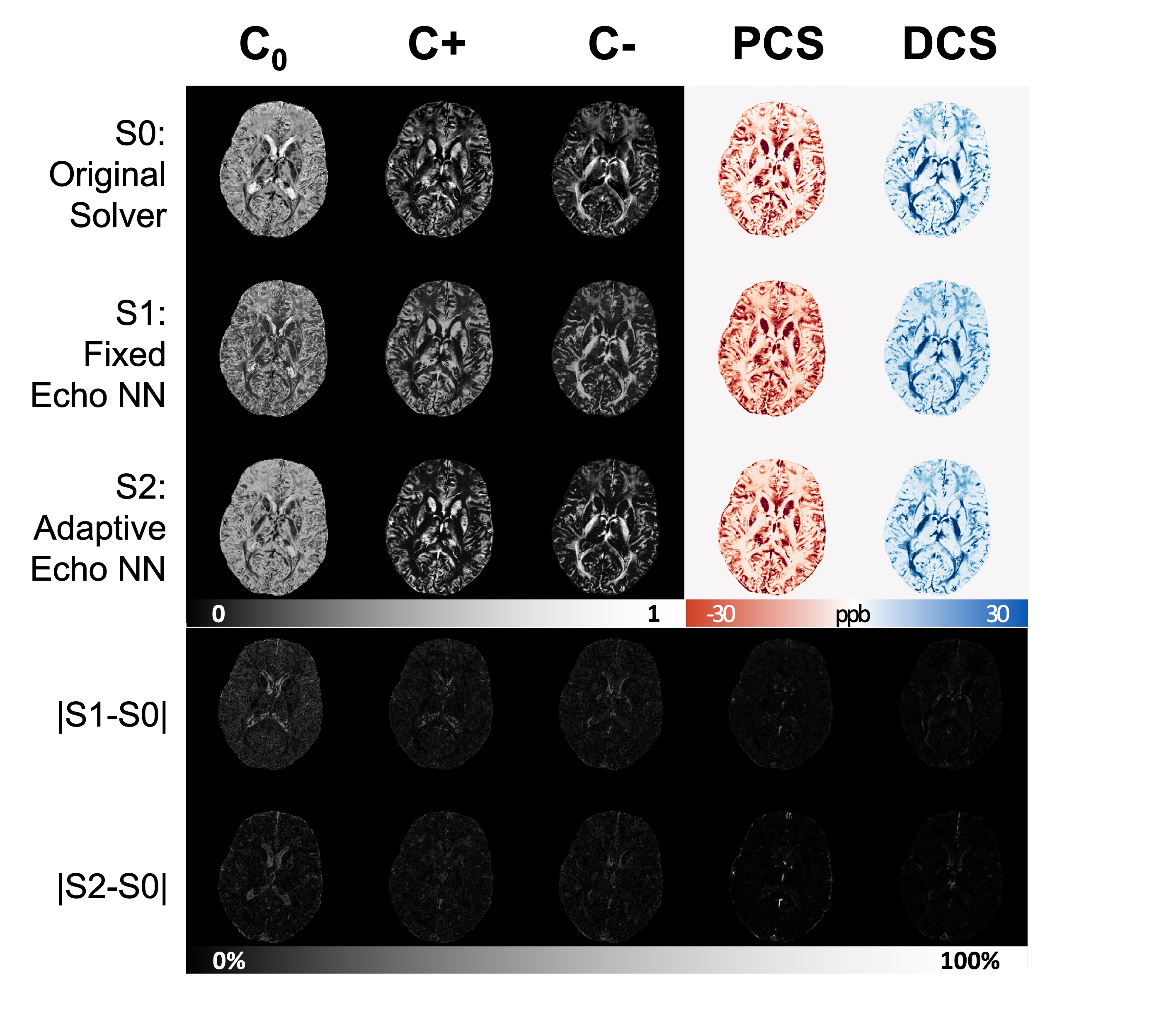
Figure 2A shows simulated signals with various echo times added with various noise levels. The model-predicted curves fit the original clean curve well. In Figure 2B, the estimated PCS and DCS from all solvers align well with the ground truth PCS and DCS. The DeepDECOMPOSE solvers show less deviation from the ground truth. Figure 3 shows the simulation results for two different noise levels and corresponding error maps. At around SNR=20, all solvers can resolve the underlying mixture to certain extent. The DeepDECOMPOSE solvers have similar performances, and both show robust performance with noisy input. With very low SNR ($$$\approx10$$$) S1 and S2 still can resolve the susceptibility mixture with less error compared to the original solver (S0). However, all solvers show difficulty when dealing with high susceptibility values. With the same data from [1], Figure 4 demonstrates the solvers' performance for the phantom data within 7 ROIs; the difference between S1, S2, and the original solver is minimal. However, the S1 results seem to have shallower contrasts. The in vivo tests (Figure 5) show that S1 and S2 achieve similar results to the original solver, with most differences occurring around the lateral ventricles. The inference time for a 256x256 image slice takes <1s on CPUs (Intel Xeon Silver 4116) and <20ms on a GPU (Nvidia Titan Xp).Discussion
We evaluate a deep learning approach for estimating DECOMPOSE-QSM. With a simple MLP implementation trained on randomly generated data, the solvers with either fixed TE (S1) or adaptive TE (S2) show the ability to perform parameter fitting for the summation of complex exponential models, specifically DECOMPOSE-QSM. The deep learning-based solvers are more than two orders of magnitude faster on CPU (four orders on GPU) than the original optimization implementation, as expected, and are more robust to measurement noise, in contrast to the original solver.We show that the spatial continuity is not compromised when training and inference in a pointwise fashion. While other network architectures can be explored, our current DeepDECOMPOSE approach is practical and readily applicable.
Acknowledgements
This work was supported in part by the Alzheimer's Drug Discovery Foundation through grant GC-201810-2017383. Research reported in this publication was in part supported by the National Institute of Aging of the National Institutes of Health under Award Number R01AG070826.
J.C. and A.D.G. contributed equally to this work.
References
[1]C. Liu, W. Li, K. A. Tong, K. W. Yeom, and S. Kuzminski, “Susceptibility-weighted imaging and quantitative susceptibility mapping in the brain: Brain Susceptibility Imaging and Mapping,” J. Magn. Reson. Imaging, vol. 42, no. 1, pp. 23–41, Jul. 2015, doi: 10.1002/jmri.24768.
[2] Y. Zhang, H. Wei, M. J. Cronin, N. He, F. Yan, and C. Liu, “Longitudinal atlas for normative human brain development and aging over the lifespan using quantitative susceptibility mapping,” NeuroImage, vol. 171, pp. 176–189, May 2018, doi: 10.1016/j.neuroimage.2018.01.008.
[3]X. Guan et al., “Regionally progressive accumulation of iron in Parkinson’s disease as measured by quantitative susceptibility mapping,” NMR in Biomedicine, vol. 30, no. 4, p. e3489, 2017, doi: https://doi.org/10.1002/nbm.3489.
[4] J. H. O. Barbosa et al., “Quantifying brain iron deposition in patients with Parkinson’s disease using quantitative susceptibility mapping, R2 and R2*,” Magnetic Resonance Imaging, vol. 33, no. 5, pp. 559–565, Jun. 2015, doi: 10.1016/j.mri.2015.02.021.
[5] N.-J. Gong, R. Dibb, M. Pletnikov, E. Benner, and C. Liu, “Imaging microstructure with diffusion and susceptibility MR: neuronal density correlation in Disrupted-in-Schizophrenia-1 mutant mice,” NMR in Biomedicine, vol. 33, no. 10, p. e4365, 2020, doi: https://doi.org/10.1002/nbm.4365.
[6] J. Chen, N.-J. Gong, K. T. Chaim, M. C. G. Otaduy, and C. Liu, “Decompose quantitative susceptibility mapping (QSM) to sub-voxel diamagnetic and paramagnetic components based on gradient-echo MRI data,” NeuroImage, vol. 242, p. 118477, Nov. 2021, doi: 10.1016/j.neuroimage.2021.118477.
[7] H.-G. Shin et al., “χ-separation: Magnetic susceptibility source separation toward iron and myelin mapping in the brain,” NeuroImage, vol. 240, p. 118371, Oct. 2021, doi: 10.1016/j.neuroimage.2021.118371.
[8] A. De Goyeneche, S. Ramachandran, K. Wang, E. Karasan, S. Yu, and M. Lustig, “ResoNet: Physics Informed Deep Learning based Off-Resonance Correction Trained on Synthetic Data,” in Proceedings of the 31st ISMRM Annual Meeting, 2022.
[9] B. S. Hu and C. Joseph Yitang, “System and method for noise-based training of a prediction model”
[10] N. Srivastava, G. Hinton, A. Krizhevsky, I. Sutskever, and R. Salakhutdinov, “Dropout: A Simple Way to Prevent Neural Networks from Overfitting,” Journal of Machine Learning Research, vol. 15, no. 56, pp. 1929–1958, 2014.
Figures
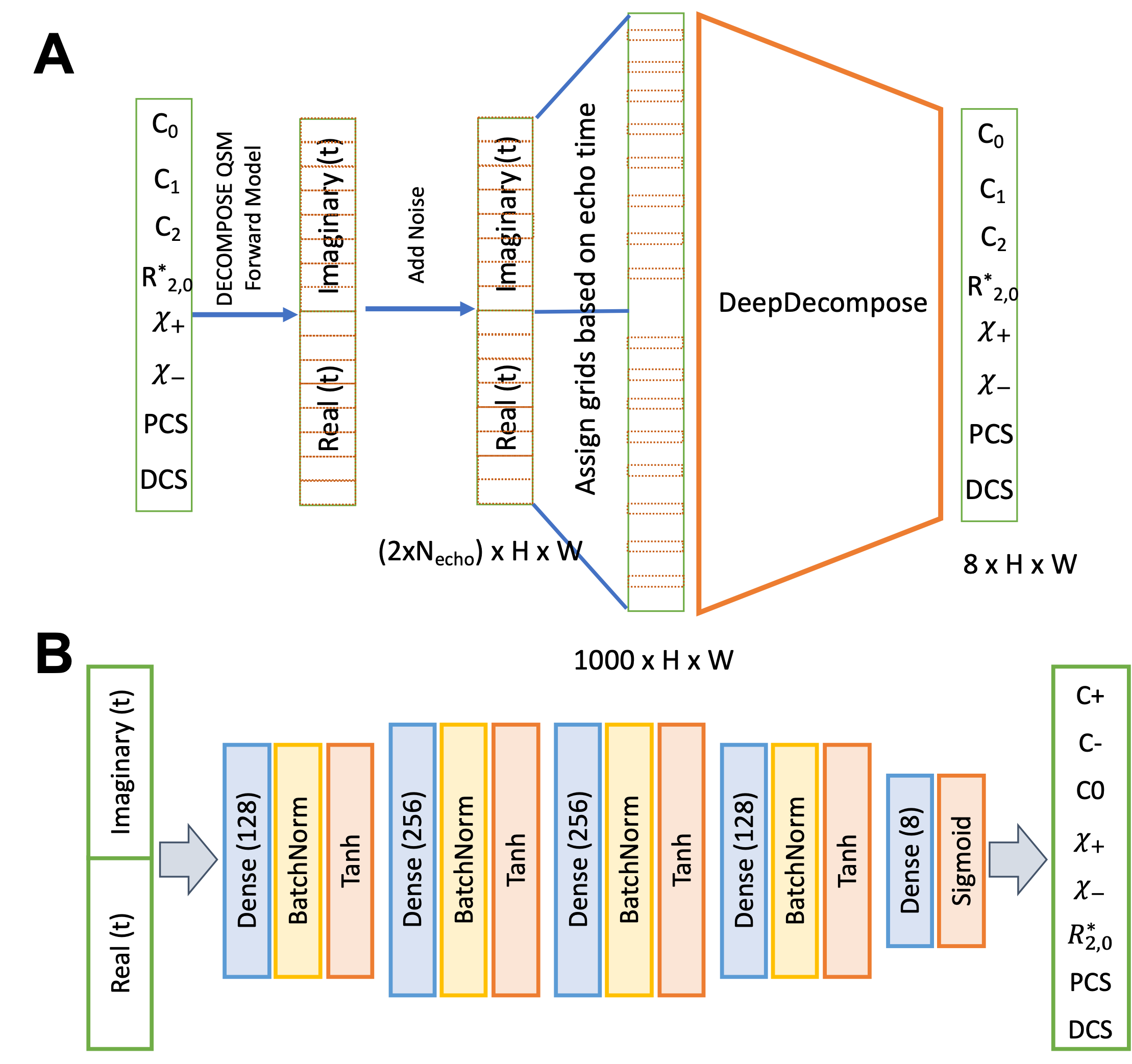
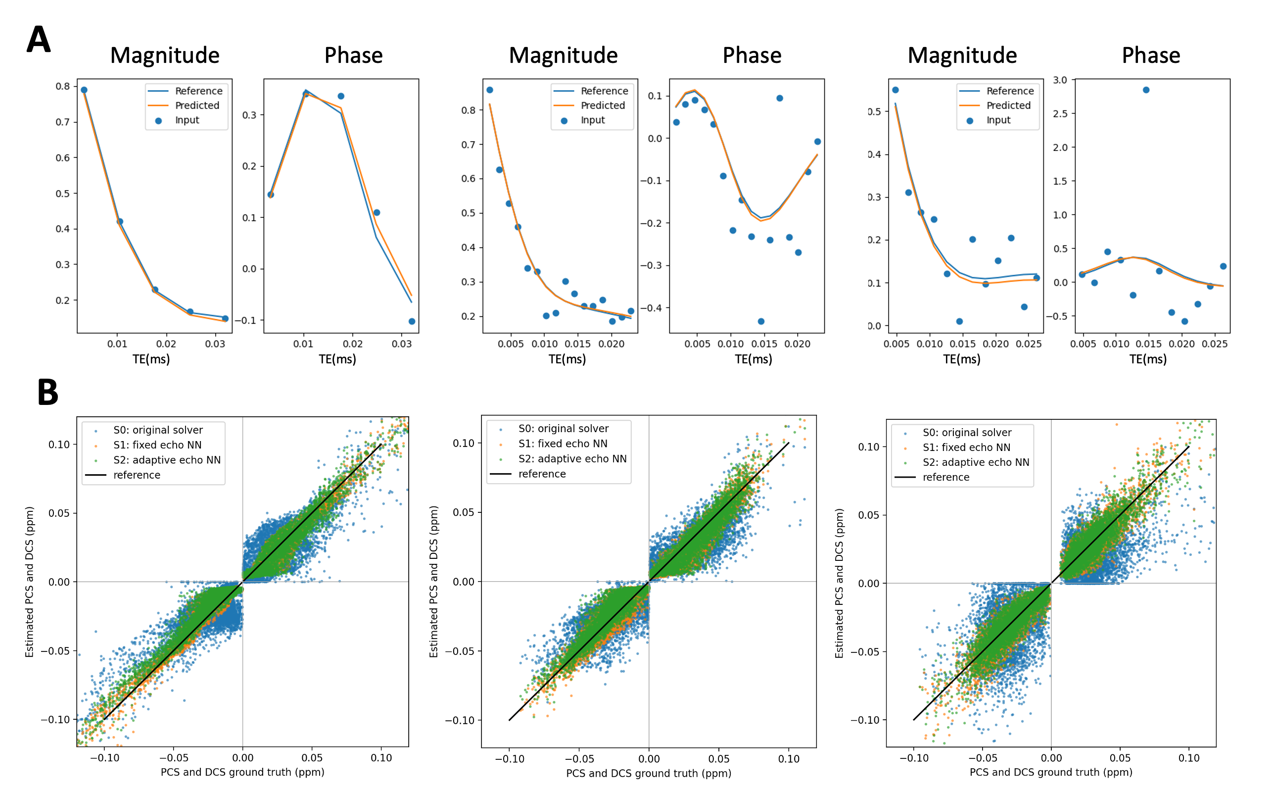
Figure 2. (A) Curve fitting performance with low, middle and high noise level and a various number of echoes. The blue curve is the clean reference. Blue scatters are the signal added with random noise, which is the input of the MLP network. The orange curve is the signal recovered from the estimated parameters outputting from the MLP network. (B) The estimated PCS and DCS from 3 solvers with low, middle and high noise level, compared to the ground truth. S1 and S2 solvers result in tighter distribution around the ground truth.