3565
An Optimized High Resolution Acquisition and Processing Pipeline for QSM in the Prostate1Dept of Medical Physics and Bioengineering, University College London, London, United Kingdom, 2Centre for Medical Imaging, University College London, London, United Kingdom
Synopsis
Keywords: Quantitative Imaging, Susceptibility, Background field removal
We aimed to optimize MRI acquisition with 1mm isotropic resolution and Quantitative Susceptibility Mapping (QSM) reconstruction for prostate clinical research. Acquisition parameters optimized in two subjects included fat-water phase artifact removal, parallel imaging acceleration factor, resolution and number of echoes. QSM masking, background field removal and susceptibility calculation were optimized in six subjects and three prostatectomy specimens. In-phase acquisition removed more fat-water phase artifacts than post-processing. VSHARP and excluding rectal gas reduced residual background fields and Iterative Tikhonov regularization reduced noise. This optimized (8.5 minute) protocol and pipeline will allow incorporation of prostate QSM in clinical research studies.
Introduction
Quantitative Susceptibility Mapping (QSM) has shown potential to measure disease-related changes in tissue iron, myelin, calcium1, 2 and oxygenation3. Prostate QSM is challenging due to large background fields induced by tissue-rectal gas interfaces 4 and fat-water phase artifacts 5. Previous prostate QSM studies 4, 6-8 have mostly used single-echo sequences, anisotropic voxels and slice thicknesses $$$\geq$$$ 1.7mm. Here, we aimed to optimize multi-echo acquisition for high-resolution scans in under 10 minutes, and a QSM pipeline, for clinical research in subjects being screened for prostate cancer.Methods
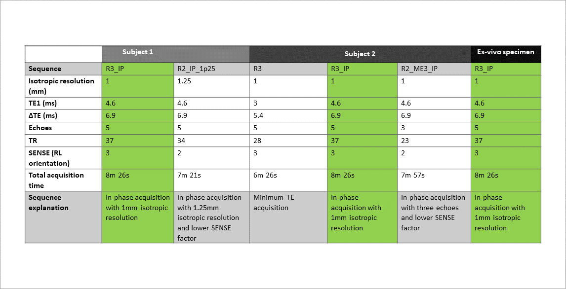
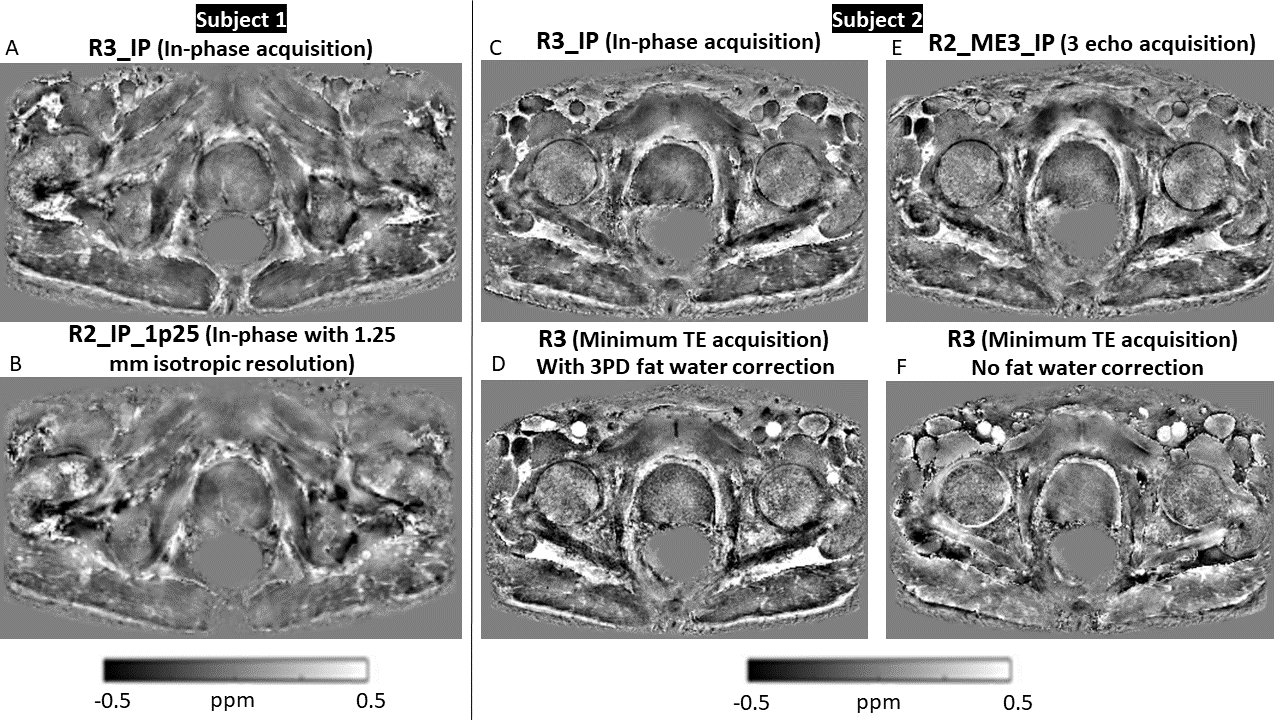
Two subjects were recruited as part of the Histo-MRI clinical study 9 and scanned on a 3T Philips Ingenia using an anterior 4x4 channel receive array and a 4x4 array in the table. All subjects were given Buscopan to reduce rectal gas and bowel motion.To optimize the SENSE factor, resolution and number of echoes, transverse multi-echo 3D-GRE images with a 420 x 320 x 128 mm field of view centered on the prostate were acquired in both subjects with the parameters in Figure 1. To optimize fat-water phase artifact removal, in-phase acquisitions 10 were compared with minimum-TE acquisition that had fat correction using a three-point Dixon (3PD) technique 11, 12. To select the optimal acquisition parameters, we made visual comparisons of susceptibility maps calculated using the optimized QSM pipeline.
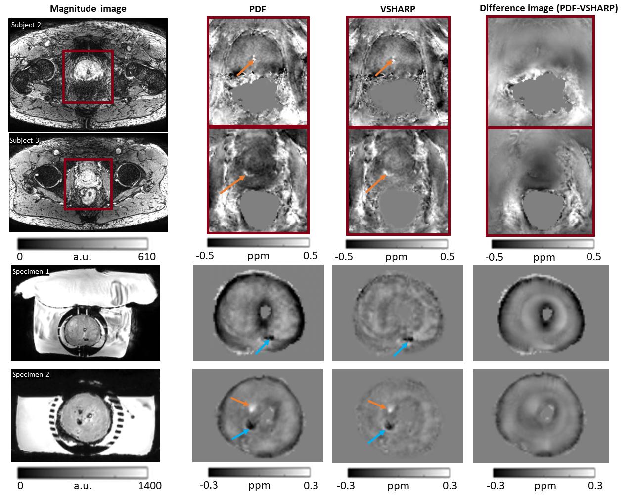
To optimize the QSM processing pipeline, the optimized parameters were used to scan four additional subjects and three Histo-MRI prostatectomy specimens preserved in formaldehyde that were placed in phosphate buffer saline (PBS) prior to scanning. In the specimens, prostate masks were manually drawn in ITK-SNAP 13, 14 on the first-echo magnitude images. Low-signal regions in a centrally placed catheter (for anatomical positioning) were removed from the mask before background field removal.
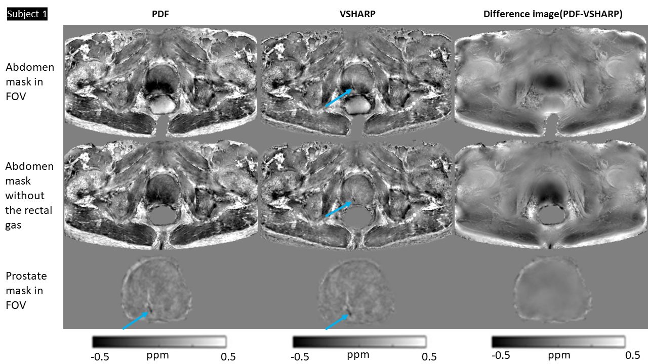
For in-vivo QSM, three masks: abdomen, abdomen without rectal gas, and prostate were compared for background field removal using Variable-radius Sophisticated Harmonic Artifact Reduction for Phase data (VSHARP)15 or Projection onto Dipole Fields (PDF) 16.
Total field maps from a non-linear fit of the complex data 17 underwent Laplacian unwrapping 18. The abdomen mask was generated by thresholding the first-echo magnitude image. As previous studies have suggested masking out gas-filled regions 4, 19, a mask of rectal gas was generated using a semi-automated method in ITK-SNAP and removed from the whole abdomen mask. The prostate mask was generated by manual segmentation in first-echo magnitude images using ITK-SNAP. Susceptibility calculation was performed using iterative Tikhonov regularization (iTik) 20 with the default regularization parameter α=0.05 and the resulting maps were visually compared.
Following background field removal with the optimized mask and VSHARP, susceptibility maps calculated with Improved Sparse Linear Equation and Least Squares (iLSQR) 21-23 and iTik 20 were visually compared. iLSQR was chosen as it had been used in previous prostate QSM studies 4, 6, 8 and iTik performed robustly in other regions 10, 24.
Results and Discussion
Susceptibility maps (Figure 2) show that 3PD correction resulted in greater noise in the prostate and some water-fat swaps relative to the in-phase acquisition which had no significant fat-water phase artifacts. The 3-echo map was noisier within the prostate than the 5-echo map despite the lower acceleration factor (R2 v. R3), probably because of the lower maximum TE resulting in lower contrast-to-noise (CNR) in the susceptibility map 25.The susceptibility maps with 1 mm isotropic resolution were sharper and seemed to have greater CNR than those with 1.25 mm isotropic resolution.Removing rectal gas from the mask reduced residual background fields in the susceptibility maps (Figure 3). VSHARP was more effective in removing residual background field artifacts than PDF although it reduced the overall susceptibility contrast. Using a prostate mask also reduced residual background fields and gave similar susceptibility maps using VSHARP and PDF. Figure 4 shows that VSHARP was more effective than PDF in removing residual background field artifacts in vivo and in specimens.
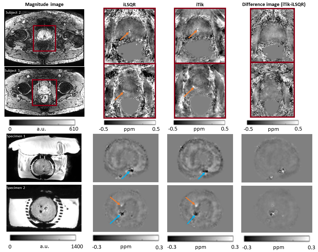
Figure 5 shows susceptibility maps calculated using iTik and iLSQR. Overall, the iLSQR maps were noisier compared to the iTik maps particularly at the edges of the prostate close to the peripheral zone. This is important as most lesions are found in the peripheral zone.
Diamagnetic regions, likely to be calcium-rich secretion residues, were observed in the prostates of several subjects (blue arrows, Figures 3, 4 and 5). Some subjects show paramagnetic regions (orange arrows, Figures 3, 4 and 5) which could indicate small haemorrhages. Future co-registration of these maps with histological stains will enable further characterization of these regions. MRI assessment of prostatic calcifications may be important in radiation therapy as calcifications could be used as markers in image guided therapy 8, 26.
Conclusion
We optimized acquisition parameters and a QSM processing pipeline for high (1mm isotropic) resolution prostate susceptibility maps acquired in < 8.5 minutes. In-phase acquisition with 5 echoes and 3-fold-SENSE acceleration provided high quality susceptibility maps in six subjects and three prostatectomy specimens. Removing rectal gas from the mask together with VSHARP background field removal reduced residual background field artifacts. iTik regularization provided high QSM CNR. This optimized protocol and pipeline will allow incorporation of QSM into clinical research studies in the prostate.Acknowledgements
This work was supported by the Cancer Research UK-EPSRC funded Multidisciplinary Project Award (award number A24348).References
1. Chen W, Zhu W, Kovanlikaya I, et al. Intracranial calcifications and hemorrhages: characterization with quantitative susceptibility mapping. Radiology 2014; 270: 496-505. 20131028. DOI: 10.1148/radiol.13122640.2. Eskreis-Winkler S, Zhang Y, Zhang J, et al. The clinical utility of QSM: disease diagnosis, medical management, and surgical planning. NMR Biomed 2017; 30 20161201. DOI: 10.1002/nbm.3668.
3. Fan AP, Bilgic B, Gagnon L, et al. Quantitative oxygenation venography from MRI phase. Magn Reson Med 2014; 72: 149-159. 20130904. DOI: 10.1002/mrm.24918.
4. Straub S, Emmerich J, Schlemmer HP, et al. Mask-Adapted Background Field Removal for Artifact Reduction in Quantitative Susceptibility Mapping of the Prostate. Tomography 2017; 3: 96-100. 2018/07/26. DOI: 10.18383/j.tom.2017.00005.
5. Dimov AV, Liu T, Spincemaille P, et al. Joint estimation of chemical shift and quantitative susceptibility mapping (chemical QSM). Magn Reson Med 2015; 73: 2100-2110. 20140619. DOI: 10.1002/mrm.25328.
6. Kan H, Tsuchiya T, Yamada M, et al. Delineation of prostatic calcification using quantitative susceptibility mapping: Spatial accuracy for magnetic resonance-only radiotherapy planning. J Appl Clin Med Phys 2021 2021/11/03. DOI: 10.1002/acm2.13469.
7. Sato R, Shirai T, Soutome Y, et al. Quantitative susceptibility mapping of prostate with separate calculations for water and fat regions for reducing shading artifacts. Magn Reson Imaging 2020; 66: 22-29. 2019/11/13. DOI: 10.1016/j.mri.2019.11.006.
8. Straub S, Laun FB, Emmerich J, et al. Potential of quantitative susceptibility mapping for detection of prostatic calcifications. J Magn Reson Imaging 2017; 45: 889-898. 2016/07/16. DOI: 10.1002/jmri.25385.
9. Singh S, Mathew M, Mertzanidou T, et al. Histo-MRI map study protocol: a prospective cohort study mapping MRI to histology for biomarker validation and prediction of prostate cancer. BMJ Open 2022; 12: e059847. 20220408. DOI: 10.1136/bmjopen-2021-059847.
10. Karsa A, Punwani S and Shmueli K. An optimized and highly repeatable MRI acquisition and processing pipeline for quantitative susceptibility mapping in the head-and-neck region. Magn Reson Med 2020; 84: 3206-3222. 20200703. DOI: 10.1002/mrm.28377.
11. ISMRM Fat-Water Separation Workshop, http://www.ismrm.org/workshops/FatWater12/ (2012).
12. Hu HH, Bornert P, Hernando D, et al. ISMRM workshop on fat-water separation: insights, applications and progress in MRI. Magn Reson Med 2012; 68: 378-388. 20120612. DOI: 10.1002/mrm.24369.
13. Yushkevich PA, Piven J, Hazlett HC, et al. User-guided 3D active contour segmentation of anatomical structures: significantly improved efficiency and reliability. Neuroimage 2006; 31: 1116-1128. 20060320. DOI: 10.1016/j.neuroimage.2006.01.015.
14. ITK-SNAP, http://www.itksnap.org/.
15. Schweser F, Deistung A, Lehr BW, et al. Quantitative imaging of intrinsic magnetic tissue properties using MRI signal phase: an approach to in vivo brain iron metabolism? Neuroimage 2011; 54: 2789-2807. 20101030. DOI: 10.1016/j.neuroimage.2010.10.070.
16. Liu T, Khalidov I, de Rochefort L, et al. A novel background field removal method for MRI using projection onto dipole fields (PDF). NMR Biomed 2011; 24: 1129-1136. 20110308. DOI: 10.1002/nbm.1670.
17. Liu T, Wisnieff C, Lou M, et al. Nonlinear formulation of the magnetic field to source relationship for robust quantitative susceptibility mapping. Magn Reson Med 2013; 69: 467-476. 20120409. DOI: 10.1002/mrm.24272.
18. Schweser F, Deistung A, Sommer K, et al. Toward online reconstruction of quantitative susceptibility maps: superfast dipole inversion. Magn Reson Med 2013; 69: 1582-1594. 20120712. DOI: 10.1002/mrm.24405.
19. Sun H, Kate M, Gioia LC, et al. Quantitative susceptibility mapping using a superposed dipole inversion method: Application to intracranial hemorrhage. Magn Reson Med 2016; 76: 781-791. 20150928. DOI: 10.1002/mrm.25919.
20. de Rochefort L, Liu T, Kressler B, et al. Quantitative susceptibility map reconstruction from MR phase data using bayesian regularization: validation and application to brain imaging. Magn Reson Med 2010; 63: 194-206. DOI: 10.1002/mrm.22187.
21. Saunders CCPaMA. LSQR: An algorithm for sparse linear equations and sparse least squares. ACM Transactions on Mathematical Software 1982; 1: 43-71.
22. Li W, Wu B and Liu C. Quantitative susceptibility mapping of human brain reflects spatial variation in tissue composition. Neuroimage 2011; 55: 1645-1656. 20110109. DOI: 10.1016/j.neuroimage.2010.11.088.
23. Li W, Wang N, Yu F, et al. A method for estimating and removing streaking artifacts in quantitative susceptibility mapping. Neuroimage 2015; 108: 111-122. 20141220. DOI: 10.1016/j.neuroimage.2014.12.043.
24. Murdoch R, Stotesbury H, Hales PW, et al. A Comparison of MRI Quantitative Susceptibility Mapping and TRUST-Based Measures of Brain Venous Oxygen Saturation in Sickle Cell Anaemia. Front Physiol 2022; 13: 913443. 20220829. DOI: 10.3389/fphys.2022.913443.
25. Biondetti E, Karsa A, Thomas DL, et al. Investigating the accuracy and precision of TE-dependent versus multi-echo QSM using Laplacian-based methods at 3 T. Magn Reson Med 2020; 84: 3040-3053. 20200603. DOI: 10.1002/mrm.28331.
26. Zeng GG, McGowan TS, Larsen TM, et al. Calcifications are potential surrogates for prostate localization in image-guided radiotherapy. Int J Radiat Oncol Biol Phys 2008; 72: 963-966. DOI: 10.1016/j.ijrobp.2008.07.021.
Figures