3486
SuperQ: 3D Super-Resolution of Quantitative Susceptibility Maps
Alexandra Grace Roberts1,2, Yi Wang1,2, Pascal Spincemaille2, and Thanh Nguyen2
1Electrical Engineering, Cornell University, Ithaca, NY, United States, 2Radiology, Weill Cornell Medicine, New York, NY, United States
1Electrical Engineering, Cornell University, Ithaca, NY, United States, 2Radiology, Weill Cornell Medicine, New York, NY, United States
Synopsis
Keywords: Machine Learning/Artificial Intelligence, Brain
3D super-resolution of QSM is feasible using the VDSR and U-net architectures using a fraction of the required number of epochs as previous 2D super-resolution networks. Additionally, this method both reduces whole brain MSE and ROI MSE and increases the apparent resolution as compared to the interpolated inputIntroduction
Quantitative Susceptibility Mapping (QSM) is a contrast in magnetic resonance imaging (MRI) that quantifies the induced magnetization of substances in the brain such as calcium deposits or iron found in blood products [1]. The sensitivity of this contrast allows the detection of microbleeds linked to COVID-19, multiple sclerosis, and vascular dementia [2]. Additionally, this quantification allows longitudinal monitoring in patients with multiple sclerosis, Parkinson’s disease [3] or Alzheimer’s disease [4]. Current clinical protocols that aim for 5-minute acquisitions are compromising spatial resolution to allow sufficient sampling of echo times. Given the compromise between resolution and acquisition time[5], [6], the use of neural networks to learn mappings between low and high-resolution images (known as super-resolution) is of interest.Generative adversarial networks (GANs) have been used to obtain super-resolved T1w images [7] and convolutional neural networks (CNNs) increase the apparent resolution of double-echo steady state (DESS) images [8] and susceptibility weighted-images (SWI) [9]. Since different contrasts in MRI visualize the same anatomical structures differently, the mappings are contrast-specific, there is benefit in examining the mapping between low and high-resolution QSM datasets. Here, the feasibility of 3D QSM super-resolution (SuperQ) is demonstrated.
Theory
The network architecture used here is a Very Deep Super Resolution (VDSR) neural network [14], the goal of which is to learn the mapping from a downsampled high-resolution image (i.e. a low-resolution image) and its residual. The residual is defined as the difference in the high-resolution image and the cubic interpolation of the downsampled image. The residual consists of features that cubic interpolation fails to represent, improving the image sharpness and overall quality. As mentioned in the original work for 2D natural images, learning the residual image rather than the high-resolution image requires less memory and allows faster convergence of stochastic gradient descent. The VDSR convergence is also compared to a U-net trained on a similar number of parameters. Training the network amounts to minimizing the mean-squared error (MSE) loss function $$E_R (θ)= \frac{1}{2} ((h_θ(x)-y)^2+\lambda(w^Tw))$$ Where $$$\theta$$$ represents network parameters, $$$h_{\theta}(x)$$$ is the learned residual between the cubic interpolation of the downsampled input $$$x$$$ and the high-resolution image $$$x_0$$$, and $$$y$$$ is the ground truth residual; $$$\lambda$$$ is an L2 regularization parameter that prevents outsized influence of a particular filter kernel in weight vector $$$w$$$. The VDSR network architecture is comprised of alternating convolution and Rectified Linear Unit (ReLU) layers with a final regression layer.Method
The network depth totals 41 layers, 20 convolution layers with filter size [3 3 3], stride of [1 1 1], and zero-padding of [1 1 1] with 20 ReLU layers. The network was initialized according to He’s method [15] and trained with a stochastic gradient descent optimizer with a momentum of 0.9 and a gradient threshold 0.1 for 100 epochs with an epoch interval 1. The batch size was 64, training was conducted with a piecewise learning schedule with initial learning rate 0.01, learning rate factor 0.1, learn rate drop period of 10 epochs and an L2 regularization factor 0.00001.Nine cases featuring 3T QSMs (of matrix size 512 x 512 x 152 and voxel size 0.43 x 0.43 x 1 mm with echo time (TE) = 20 ms) were acquired and split 7:1:1 into training, testing, and validation subsets. Training and validation sets were divided into 16 x 16 x 32 patches, which was found to be the optimal size via grid search. The training volume was downsampled using k-space cropping by a factor of 2, 3, and 4. The downsampled volume was cubically interpolated (upsampled) by the same factor. The residual was calculated by subtracting the cubic interpolation from the initial high-resolution. The MSE and apparent resolution [16] between the ground truth and super-resolved image (the sum of the cubic interpolation and residual) was calculated on the brain volume and regions of interest (ROIs) - the red nucleus, substantia nigra, caudate nucleus, globus pallidus, dentate nucleus, and putamen. A U-net with a similar number of parameters was trained for 50 epochs for comparison. A test cast outside the (healthy subjects) training distribution consisting of a patient with multiple sclerosis (MS) was evaluated.
Results
SuperQ demonstrates lower MSE in the whole brain volume and ROIs as shown in Table 1. The improvement in the visual quality of the test case is shown (Figures 1, 2). A U-net architecture with a smaller set of parameters outperformed the VDSR architecture after 50 epochs of training (Figure 3). The improved performance by the U-net may offer insight into the quantitative super-resolution problem. Additionally, SuperQ is trained on 3D data and requires less than a 10th of the number of epochs in the previously proposed 2D method and generalizes to a case outside the training distribution (Figure 4).Discussion
3D super-resolution of QSM is feasible using the VDSR and U-net architectures using a fraction of the required number of epochs as 2D super-resolution networks. Additionally, this method reduces whole brain and ROI MSE and increases the apparent resolution compared to the interpolated input. Learning the residual rather than the high-resolution image grants generalization to the mapping, as is seen with the MS case. Future work includes k-space domain training and prospective super-resolution.Acknowledgements
No acknowledgement found.References
- Wang, Y. and T. Liu (2015). "Quantitative susceptibility mapping (QSM): Decoding MRI data for a tissue magnetic biomarker." Magnetic Resonance in Medicine 73(1): 82-101.
- M. Ayaz, A. S. Boikov, E. M. Haacke, D. K. Kido, and W. M. Kirsch, “Imaging cerebral microbleeds using susceptibility weighted imaging: one step toward detecting vascular dementia: Imaging Microbleeds Using SWI,” J. Magn. Reson. Imaging, vol. 31, no. 1, pp. 142–148, 2010.
- Du, G., et al. (2016). "Quantitative susceptibility mapping of the midbrain in Parkinson's disease." Movement Disorders 31(3): 317-324.
- Kim, H.G., et al. (2017). "Quantitative susceptibility mapping to evaluate the early stage of Alzheimer's disease." NeuroImage. Clinical 16: 429-438.
- M. Kozak, C. Jaimes, J. Kirsch, and M. S. Gee, “MRI techniques to decrease imaging times in children,” Radiographics, vol. 40, no. 2, pp. 485–502, 2020.
- J. Yeung, “Spatial resolution (MRI),” Radiopaedia.org. [Online]. Available: https://radiopaedia.org/articles/spatial-resolution-mri-2?lang=us. [Accessed: 28-Sep-2021].
- Y. Chen, A. G. Christodoulou, Z. Zhou, F. Shi, Y. Xie, and D. Li, “MRI super-resolution with GAN and 3D multi-level DenseNet: Smaller, faster, and better,” arXiv [cs.CV], 2020.
- A. S. Chaudhari et al., “Super‐resolution musculoskeletal MRI using deep learning,” Magn. Reson. Med., vol. 80, no. 5, pp. 2139–2154, 2018.
- A.G. Roberts, P. Spincemaille, I. Kovanlikaya, John T., T. Nguyen, and Y. Wang. SWISeR: Multi-field susceptibility-weighted images super-resolution. In Proceedings of International Society for Magnetic Resonance in Medicine, 2022
- K. Zeng, H. Zheng, C. Cai, Y. Yang, K. Zhang, and Z. Chen, “Simultaneous single- and multi-contrast super-resolution for brain MRI images based on a convolutional neural network,” Comput. Biol. Med., vol. 99, pp. 133–141, 2018.
- S. Roy, A. Jog, E. Magrath, J. A. Butman, and D. L. Pham, “Cerebral microbleed segmentation from susceptibility weighted images,” in Medical Imaging 2015: Image Processing, 2015.
- B. Bachrata, S. Bollmann, G. Grabner, S. Trattnig, and S. Robinson Isotropic QSM in seconds using super-resolution 2D EPI Imaging in 3 Orthogonal Planes. In Proceedings of International Society for Magnetic Resonance in Medicine, 2022.
- A. Moevus, M. Dehaes, B. De Leener. Improving Deep Learning MRI Super-Resolution for Quantitative Susceptibility Mapping. International Society for Magnetic Resonance Imaging, Magnetic Resonance in Medicine, 2021.
- J. Kim, J. K. Lee, and K. M. Lee, “Accurate image super-resolution using very deep convolutional networks,” arXiv [cs.CV], 2015.
- He, K., et al. Delving Deep into Rectifiers: Surpassing Human-Level Performance on ImageNet Classification, IEEE.
- Eskreis-Winkler S, Zhou D, Liu T, Gupta A, Gauthier SA, Wang Y, Spincemaille P. On the influence of zero-padding on the nonlinear operations in Quantitative Susceptibility Mapping. Magn Reson Imaging. 2017 Jan;35:154-159. doi: 10.1016/j.mri.2016.08.020. Epub 2016 Aug 29. PMID: 27587225; PMCID: PMC5160043.
Figures
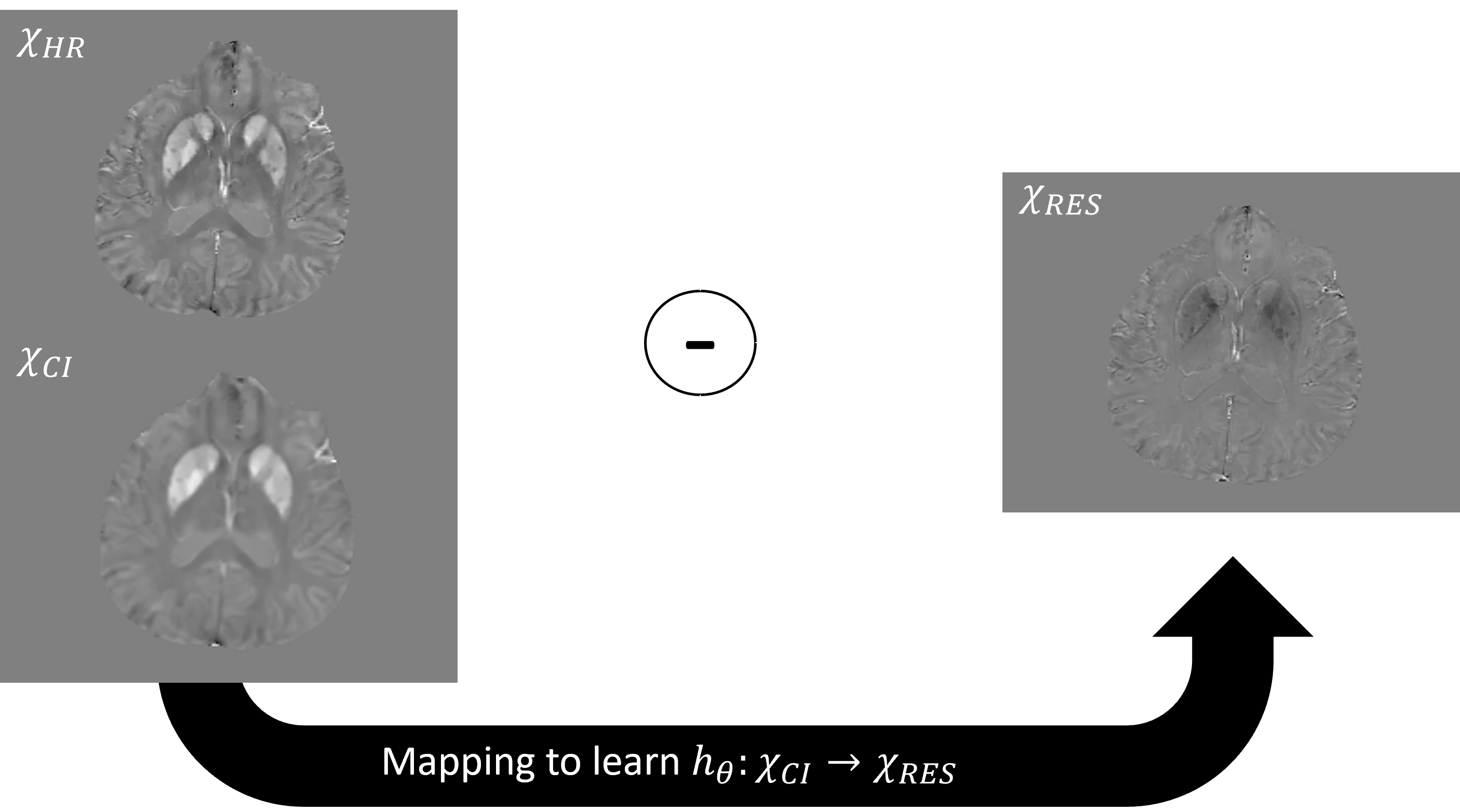
Figure 1. The learned residual mapping.
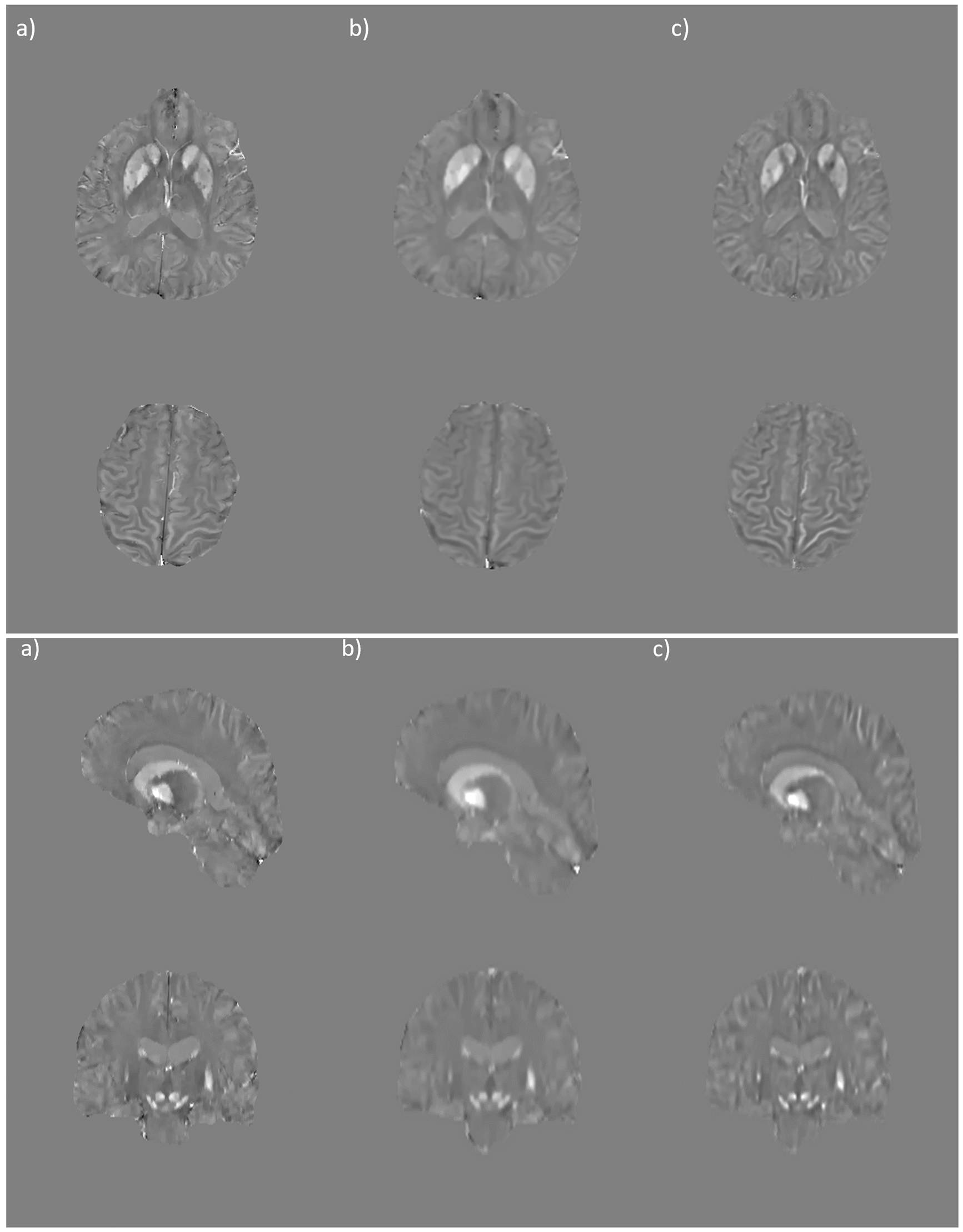
Figure 2. Ground truth (a), interpolated (b), and super-resolved (c) QSM. Note the
improved demarcation of the caudate nucleus, putamen, and globus pallidus not
visible in the interpolation.
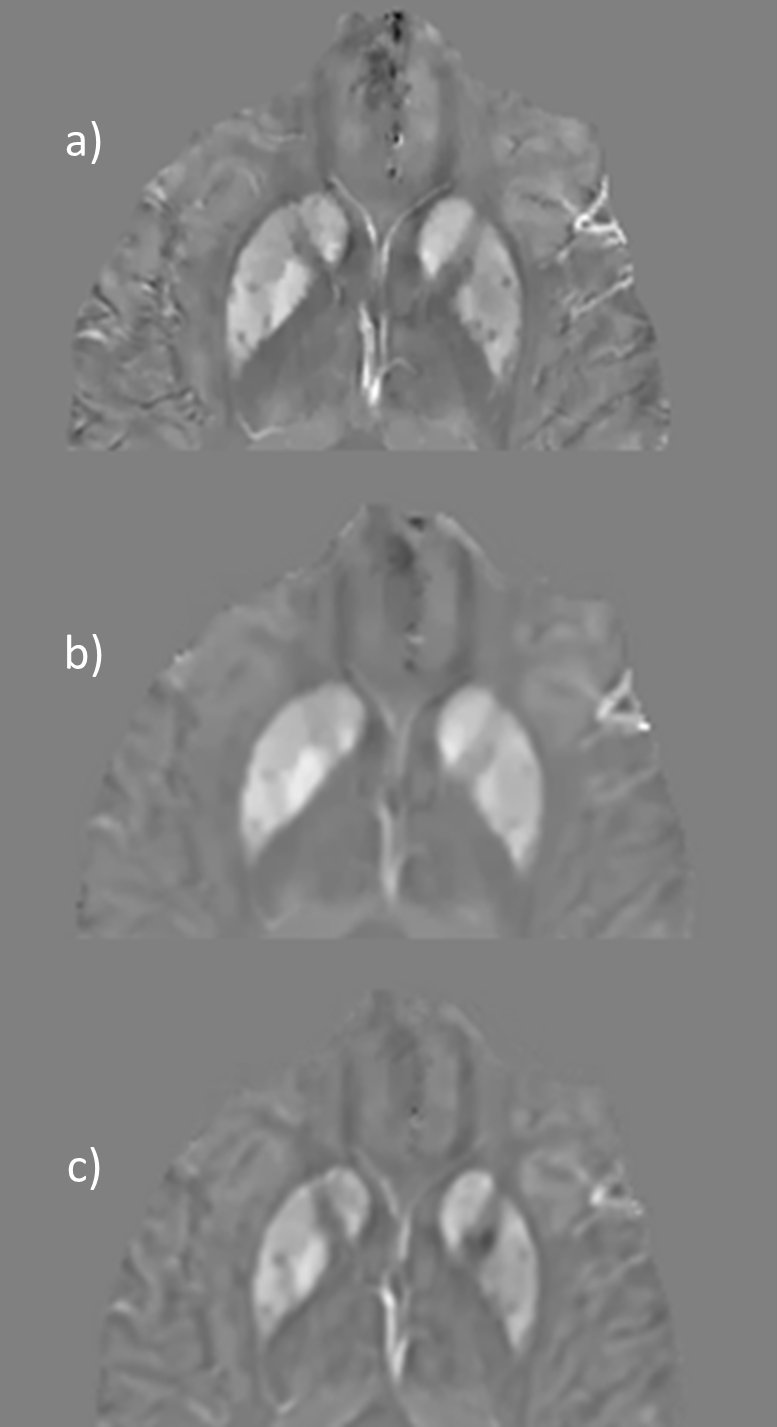
Figure 3. Ground truth (a), interpolated
(b), and super-resolved (c) QSM, 2x view.
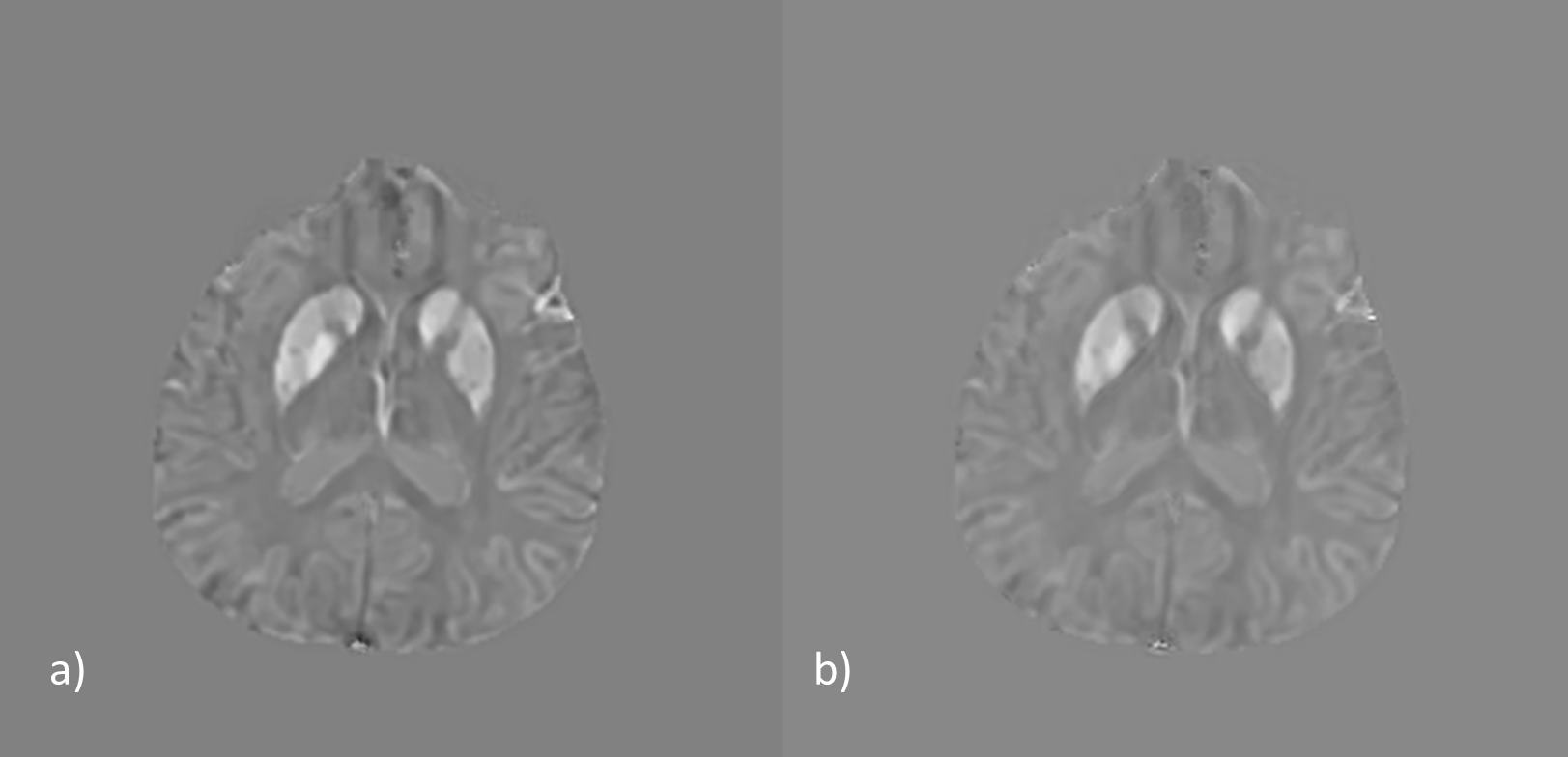
Figure 4. U-net (left) and
VDSR (right) comparison after 50 epochs, the U-net to converge more quickly.
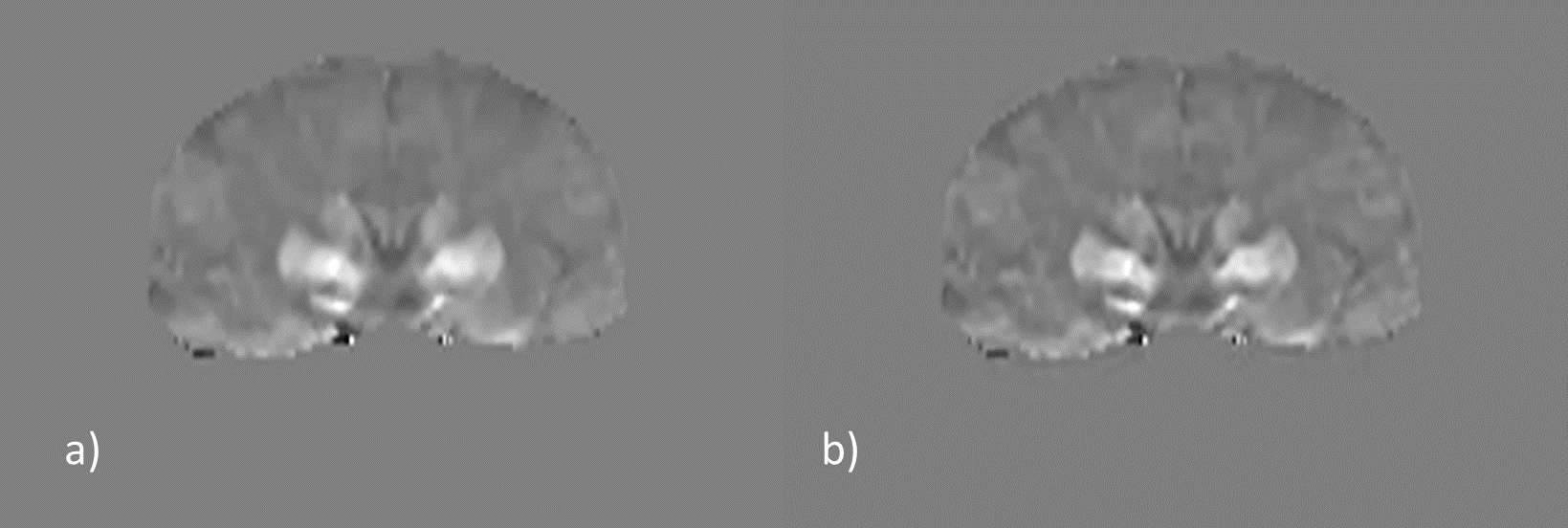
Figure 5. Learning the residual allows improvement of an
MS case (a) after super-resolution (b) outside the training distribution.
DOI: https://doi.org/10.58530/2023/3486