3482
A new directional colormap for DTI fiber tractography and its application to bundle recognition
Mauro Zucchelli1, Christos Papageorgakis1, and Stefano Casagranda1
1Department of R&D Advanced Applications, Olea Medical, La Ciotat, France
1Department of R&D Advanced Applications, Olea Medical, La Ciotat, France
Synopsis
Keywords: Brain Connectivity, Tractography & Fibre Modelling, Colormap, Diffusion
We propose a new tractography colormap based on the HSL model to complement the classical RGB colormap used in the field. Our colormap is based on a new feature, called "streamlines normal", an oriented vector that is computed from the tractography. The streamlines normal in combination with the HSL colormap improves tractography data visualization and can be an asset for better and faster bundle segmentation both manually and automatically.INTRODUCTION
Diffusion MRI tractography1 is widely used to probe brain fiber connections both in clinical practice and on healthy subjects. In addition, diffusion tractography can aid the identification of healthy tracts that lie in the proximity of a target region2, which could be beneficial for some tumor cases and drug-resistant types of epilepsy, where surgical removal of a part of the brain is required. Researchers have designed numerous algorithms for the automatic labeling of tractography streamlines3, mapping them to known anatomical bundles, but in several hospitals, this operation is still performed manually by experts. In the current standard, tractography streamlines are visualized with a color coding method that aims at encoding the main streamline directions. Streamlines going anterior-posterior are colored green, vertical streamlines going dorsal-ventral are colored blue, and streamlines going left-right are colored red. However, the RGB color representation does not exploit the color space completely.We are proposing a new colormap for tractography streamlines based on the Hue Saturation Lightness (HSL) color model. Since streamline directions do not have an orientation, we also introduce a new directional feature, called “streamline normal” that complements the streamline direction. The streamlines normals can be used as a feature for improving the current automatic bundle segmentation algorithms and the combination of the normal with the HSL colormap makes the tractography easier to interpret and segment for human operators.METHODS
In order to calculate the streamlines normal, we first resample each streamline as an Nx3 array of 3D points, with N=31. We call the starting point of the streamline A and the last point B (see Figure 1). We define the streamline normal as the vector v [P, AB] having the following properties: i) v starts from a streamline point P and ends along the vector AB, ii) v is perpendicular to AB, and iii) |v|, the distance between the P and AB, reaches its maximum. Figure 1 shows a graphical representation of the vector v (dashed line) for a generic streamline (colored in blue). Contrary to the main streamlines direction, the streamlines normal are oriented vectors and therefore can benefit from a more detailed color representation. HSL has been used as an alternative color base for RGB for decades in the computer graphics community. Considering the elevation and azimuth angle of v in spherical coordinates, namely θ ([0, π] range) and φ ([0, 2π]). We consider H=φ and L=1.0-θ/π. Regarding the saturation, we consider either i) a saturation of one, where all streamlines are fully saturated or ii) we set the saturation to the curvature of the streamline calculated as S=|AB|/length(streamline). In the latter case, the more a streamline follows a straight line the higher its saturation. This parametrization stems from the empirical observation that spurious streamlines, which can be considered tractography artifacts, are generally more curved and tortuous than real axonal pathways.RESULTS
Figure 2 (left) shows a coronal view of a DTI FACT tractography of a healthy human brain, colored with the classical RGB model. For visualization purposes, we show only streamlines with lengths in the range of 50-200 mm, for a total of 17000 streamlines. Figure 2 (central and right) shows the same tractography colored with the HSL model with S=1 and curvature-dependent S, respectively. An axial view of the same tractography is presented in Figure 3. The HSL colormap highlights several important bundles such as the corticospinal tracts (left and right) the different segments of the corpus callosum (CC), and the arcuate fasciculus (AF). Having the saturation S depending on the curvature (right figures) highlights the straighter streamline bundles like the corticospinal tract (CST) or the fronto-occipital fasciculi (FOF).To demonstrate the differences with respect to the classical RGB map, we select three subsets of streamlines each aligned with the main cartesian axes. Figure 4, shows the streamlines aligned in the x, y, and z directions, respectively, in each row. Each subset is selected to fall into a cone of 25 degrees with respect to the chosen direction. The streamlines aligned in the x directions belong mostly to the CC and while they appear as uniform red in RGB the different sub-bundles are perfectly distinguishable with the HSL colormap. The y-streamlines (green in RGB) are more heterogeneous and are composed of streamlines of the cingulum, AF, and inferior FOF. The z-streamlines (blue in RGB) mostly belong to the CST and the HSL colormap allowing us to distinguish between the left and right parts of the bundle.DISCUSSION and CONCLUSION
Manual streamline segmentation is time-consuming and becomes exponentially more difficult with the increase in the number of streamlines in the tractography. The color information present in the HSL colormap, calculated using the streamlines normal, helps to differentiate between the different fiber bundles and complements the directional information of the classical RGB colormap. The streamline normal can also be used as a numerical feature to improve existing streamline-clustering algorithms or to design new ones which will be studied in our future work.Acknowledgements
No acknowledgement found.References
[1] Basser, Peter J., et al. In vivo fiber tractography using DT‐MRI data. Magnetic resonance in medicine, 2000, 44.4: 625-632.
[2] Berman, Jeffrey. Diffusion MR tractography as a tool for surgical planning. Magnetic resonance imaging clinics of North America, 2009, 17.2: 205-214.
[3] Garyfallidis, Eleftherios, et al. Quickbundles, a method for tractography simplification. Frontiers in neuroscience, 2012, 6: 175.
Figures
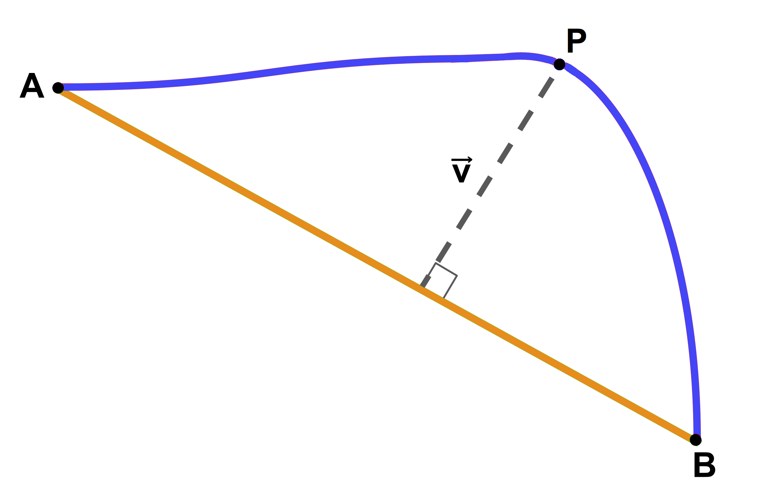
Figure 1. Graphical representation of a streamline normal v (dashed line) for a generic streamline (blue curve). Point A and B represent the starting and ending points of the streamline and point P is the point of the streamline having the maximum distance from the vector AB.
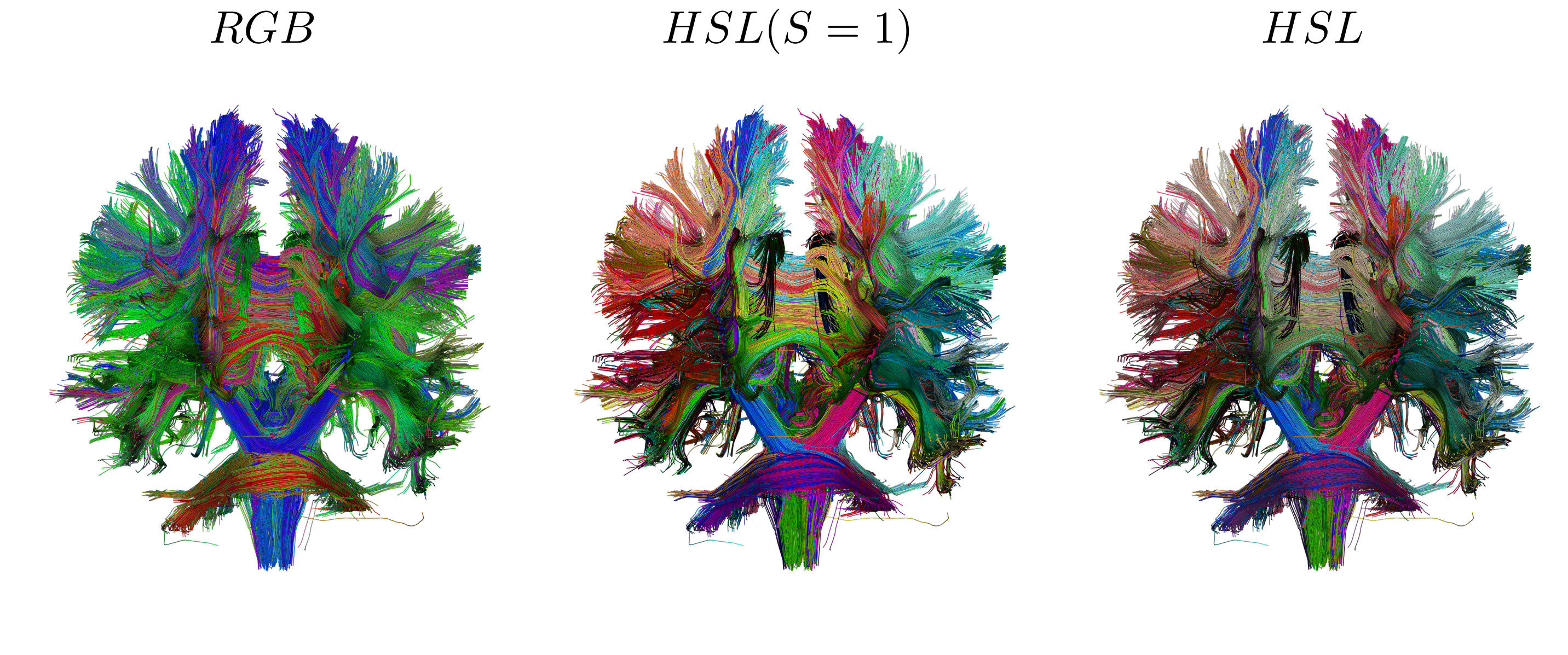
Figure 2. A coronal view of a DTI FACT tractography of a healthy human brain, colored with the classical RGB colormap (left), with our HSL colormap setting S=1 (center), and with the HSL colormap with S depending on the streamline curvature.
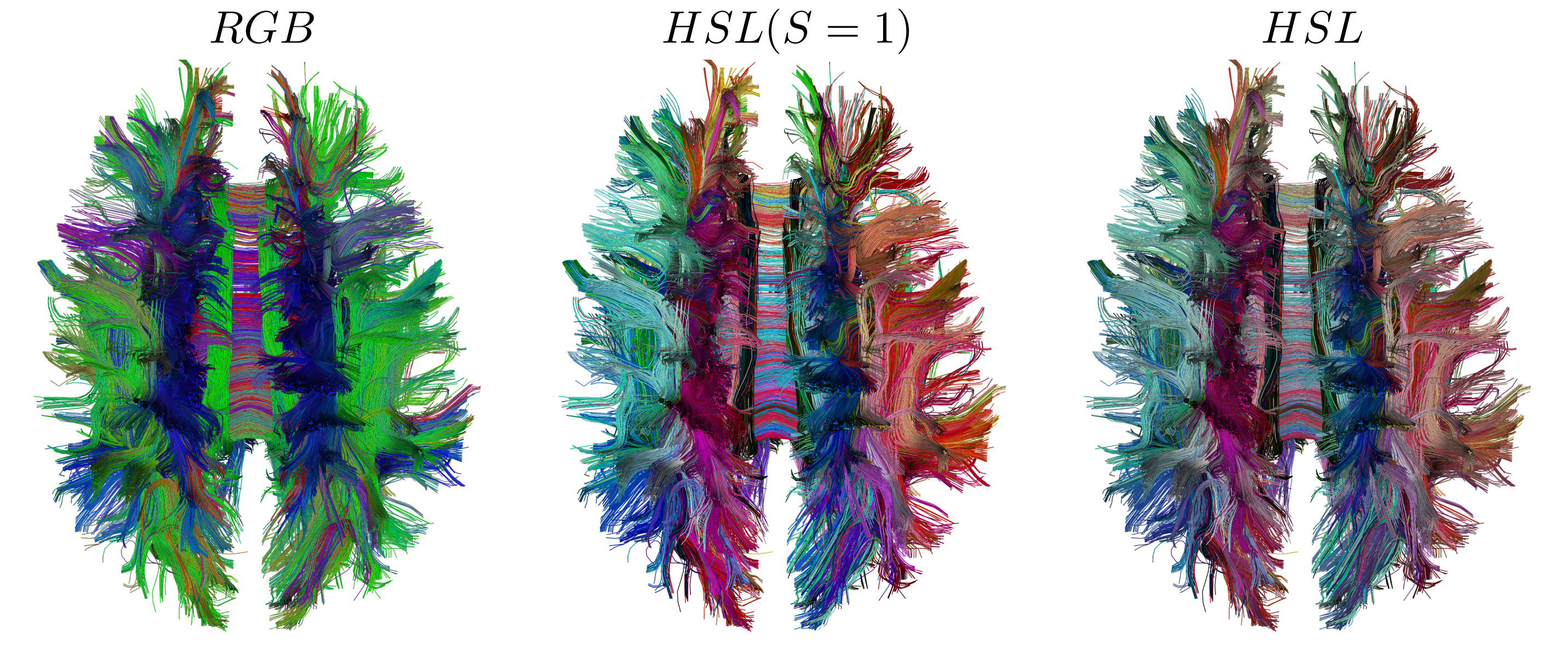
Figure 3. An axial view of a DTI FACT tractography of a healthy human brain, colored with the classical RGB colormap (left), with our HSL colormap setting S=1 (center), and with the HSL colormap with S depending on the streamline curvature.
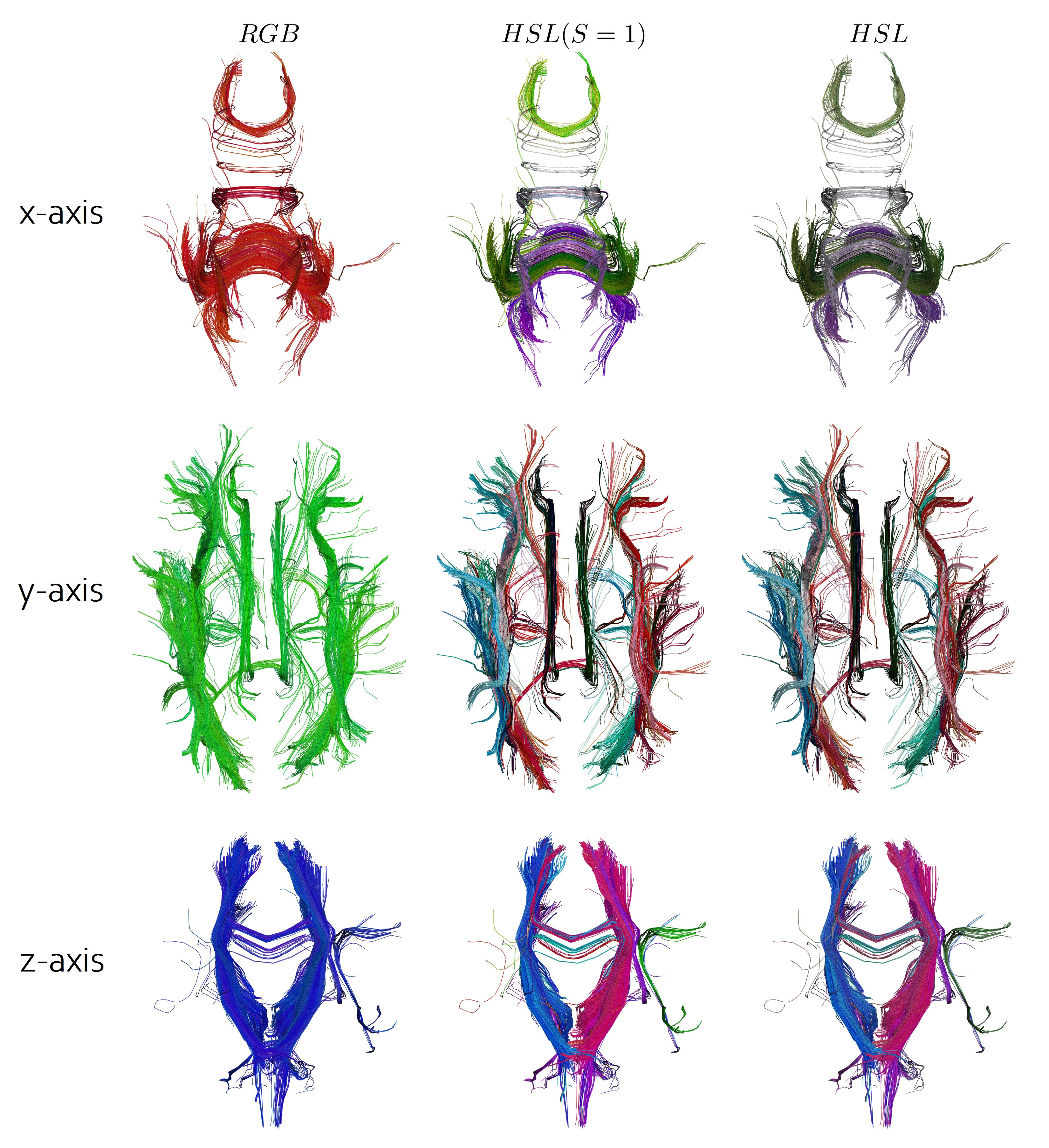
Figure 4. Subset of tractography streamlines aligned in the x, y, and y direction, respectively, in each row. The left column is colored with the classical RGB colormap, the central with our HSL colormap setting S=1, and the right with the HSL colormap with S depending on the streamline curvature.
DOI: https://doi.org/10.58530/2023/3482