3434
Performance of Multipool Lorentzian fitting for CEST-MRI using joint spatial regularization1Institute of Biomedical Imaging, Graz University of Technology, Graz, Austria, 2Institute of Neuroradiology, Friedrich-Alexander-Universität Erlangen-Nürnberg (FAU), University Hospital Erlangen, Erlangen, Germany, 3Institute of Mathematics and Scientific Computing, University of Graz, Graz, Austria, 4High-Field Magnetic Resonance Center, Max-Planck Institute for Biological Cybernetics, Tübingen, Germany, 5BioTechMed Graz, Graz, Austria
Synopsis
Keywords: Data Analysis, CEST & MT
This work investigates an improved quantification algorithm for CEST spectra using a joint Frobenius TGV regularization. The performance is assessed with simulations, phantom and in-vivo measurement with respect to systematic errors and robustness. For comparison, a pixel-wise fit using the Levenberg-Marquardt algorithm and the IDEAL algorithm were implemented. The $$$TGV_j$$$ algorithm shows the best performance in the main parameter fitting stability and parameter SNR.Introduction
The Chemical Exchange Saturation Transfer (CEST) contrast allows the detection of specific molecular information, by using the exchange between solute pools and free water to amplify the signal1. A common analysis technique of the resulting Z-Spectrum is Multipool-Lorentzian-fitting, where multiple Lorentzian-functions are fitted to the spectrum to quantify individual contributions1. This approach suffers from the poor SNR of CEST images and the limited number of offset frequencies, both caused by limitations to the acquisition time. Those limitations, combined with the high number of parameters used in the fit, can lead to unstable results and noisy parameter maps. Recently an approach using joint spatial TGV-regularization ($$$TGV_j$$$) was proposed to improve the SNR and the stability of nonlinear parameter mapping2,4. This work now investigates the $$$TGV_j$$$-regularization with respect to systematic errors and robustness using simulations and measurements. The new approach is compared to a standard nonlinear fit using the Levenberg-Marquardt algorithm as well as a method called the “Image Downsampling Expedited Adaptive Leastsquares” (IDEAL) algorithm3.Theory
In Multipool-Lorentzian-fitting each pool is described by$$L_i(\omega) = a_i \frac{{(\Gamma_i/2)}^2}{{(\Gamma_i/2)}^2 + (\omega - \omega_{0i})}$$
where $$$\omega$$$ describes the offset frequency, $$$a_i$$$ the amplitude, $$$\Gamma_i$$$ the width and $$$\omega_{0i}$$$ the shift of the lineshape.
To incorporate spatial regularization, the following non-linear problem is solved:
$$\min_x||A(x)-d||^2_2+\lambda TGV_j(x),$$
where $$$A$$$ is the non-linear forward operator mapping parameter maps to complex data using the Lorentian lineshapes, $$$x=[a_0,...,a_n,\Gamma_0,...,\Gamma_n,\omega_0,...,\omega_n]$$$ is the parameter-vector, $$$d$$$ is the acquired data and $$$\lambda>0$$$ is the weighting parameter for the joint-total-generalized-variation ($$$TGV_j$$$)2,4,5.
The IDEAL fitting approach was first proposed by Zhou et al. in 20173. IDEAL fits down sampled versions of the images to acquire starting values for a pixel-wise fit. The fit is then solved with tight boundaries ($$$\pm10\%$$$), which limits the amount of variance from the start values.
Methods
A numerical phantom was constructed in MATLAB (2021a,MathWorks,Natick,MA), based on an anatomical model, from the MRiLab-toolbox6. An artificial tumor was added as a 3D ellipsis. A Gaussian filter was applied to the tissue labels to simulate partial volume effects and transitions between tissues. The spectrum was simulated for each tissue type (Cerebrospinal fluid (CSF), white matter (WM), gray matter (GM) and two types of the Glioma tissue (GLIO)) by modeling measured data using a five pool model in pulseq-cest7. The simulated spectra were then used to generate an image series based on the altered anatomical model. The image series was converted to k-space and Gaussian noise was added to match the SNR (52dB for the reference image) of the measured data.A three pool phantom containing water, $$$Mn_2Cl$$$, Creatine and Nicotinamid was measured using a MAGNETON Vida 3T scanner (Siemens Healthcare GmbH,Erlangen,Germany). The sequence was build in house using pulseq-cest7 with a pulsed Gaussian saturation followed by a centric 2D-GRE readout with parameters: base resolution = $$$64\times64$$$, FOV = $$$160\times160$$$ $$$mm^2$$$, slice thickness 5$$$mm$$$, $$$\alpha=10^{\circ}$$$, $$$T_R=12ms$$$ and $$$T_E=4ms$$$.
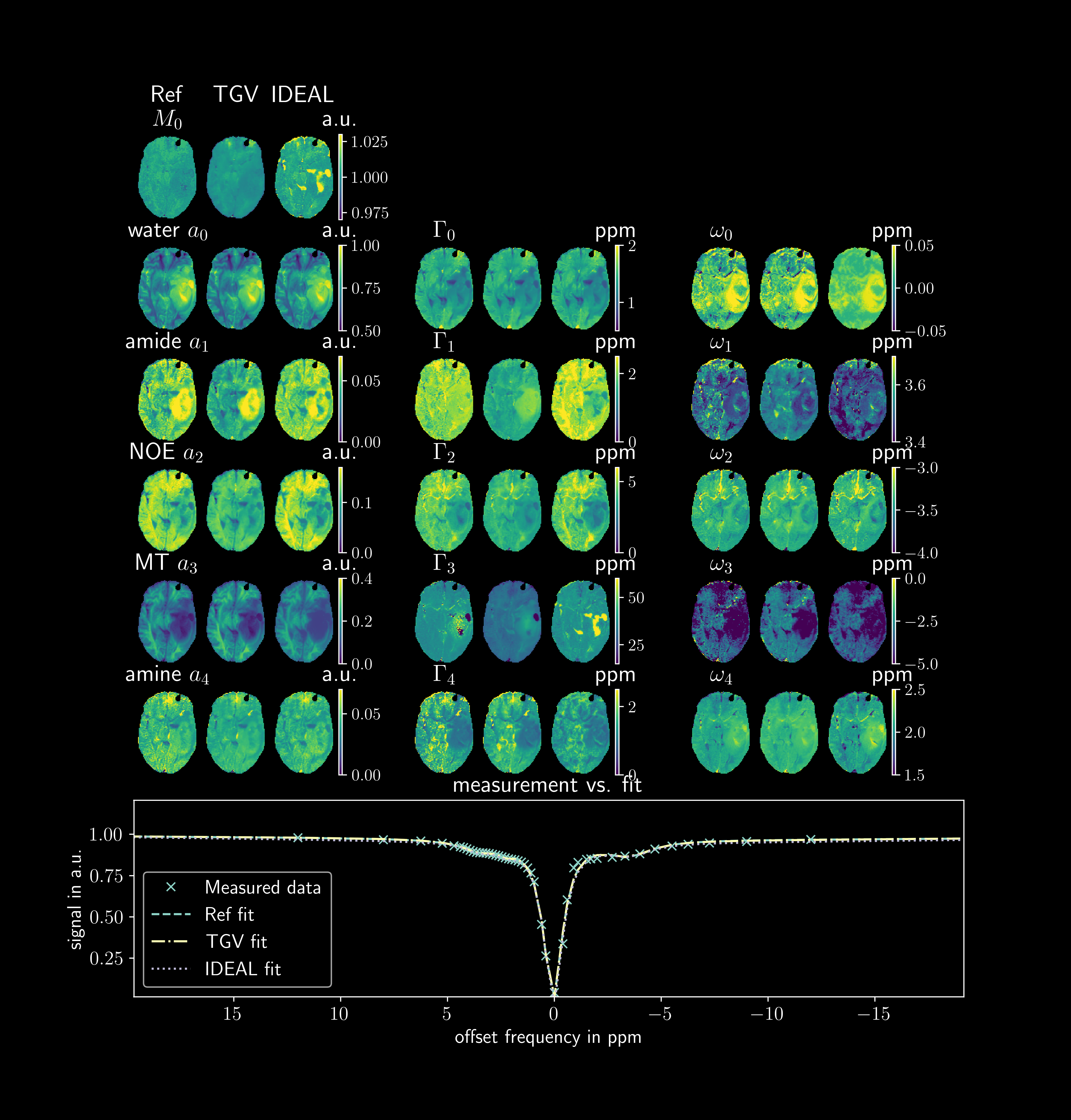
In-vivo data was acquired using a MAGNETOM Terra 7T scanner (Siemens Healthcare GmbH,Erlangen,Germany) using the MIMOSA scheme8 for pre-saturation followed by a readout using a centric 3D snapshot GRE with parameters: base resolution=$$$104\times128\times18$$$, FOV=$$$230\times186.875\times23$$$ $$$mm^3$$$, $$$\alpha=6^{\circ}$$$, $$$T_R=3700ms$$$ and $$$T_E=1770ms$$$9. The measured data was motion corrected, denoised and corrected for $$$B_1^+$$$.
Parameter fitting was performed using the MATLAB function lsqcurvefit for the conventional pixel-wise fit and the PyQMRI-toolbox10 in Python for the TGV-fit. PyQMRI uses the iteratively-regularized-Gauss-Newton (IRGN) method combined with a primal-dual splitting algorithm to solve the non-linear problem10,11. The IDEAL fitting approach was implemented in MATLAB using lsqcurvefit.
Results and Discussion
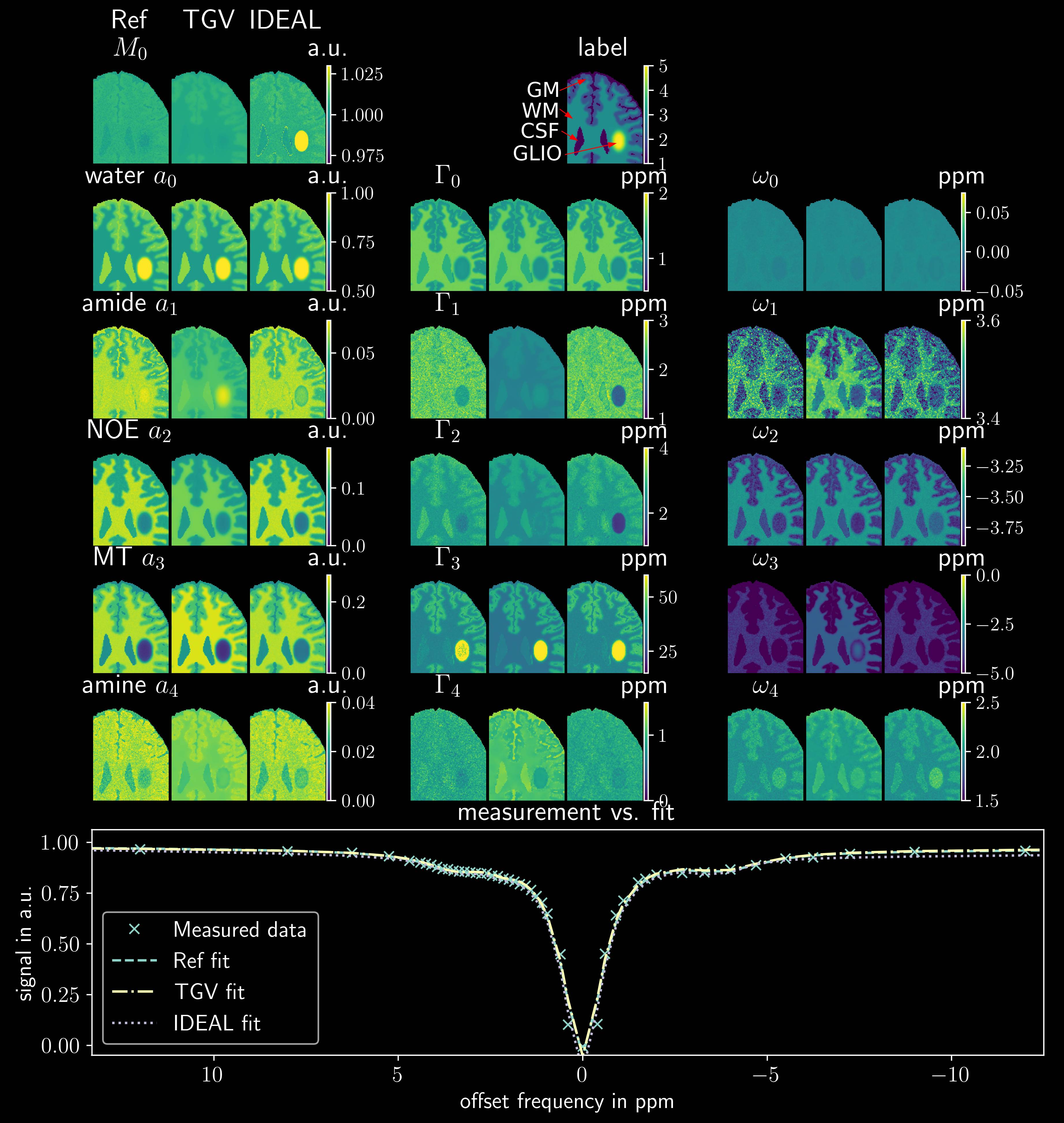
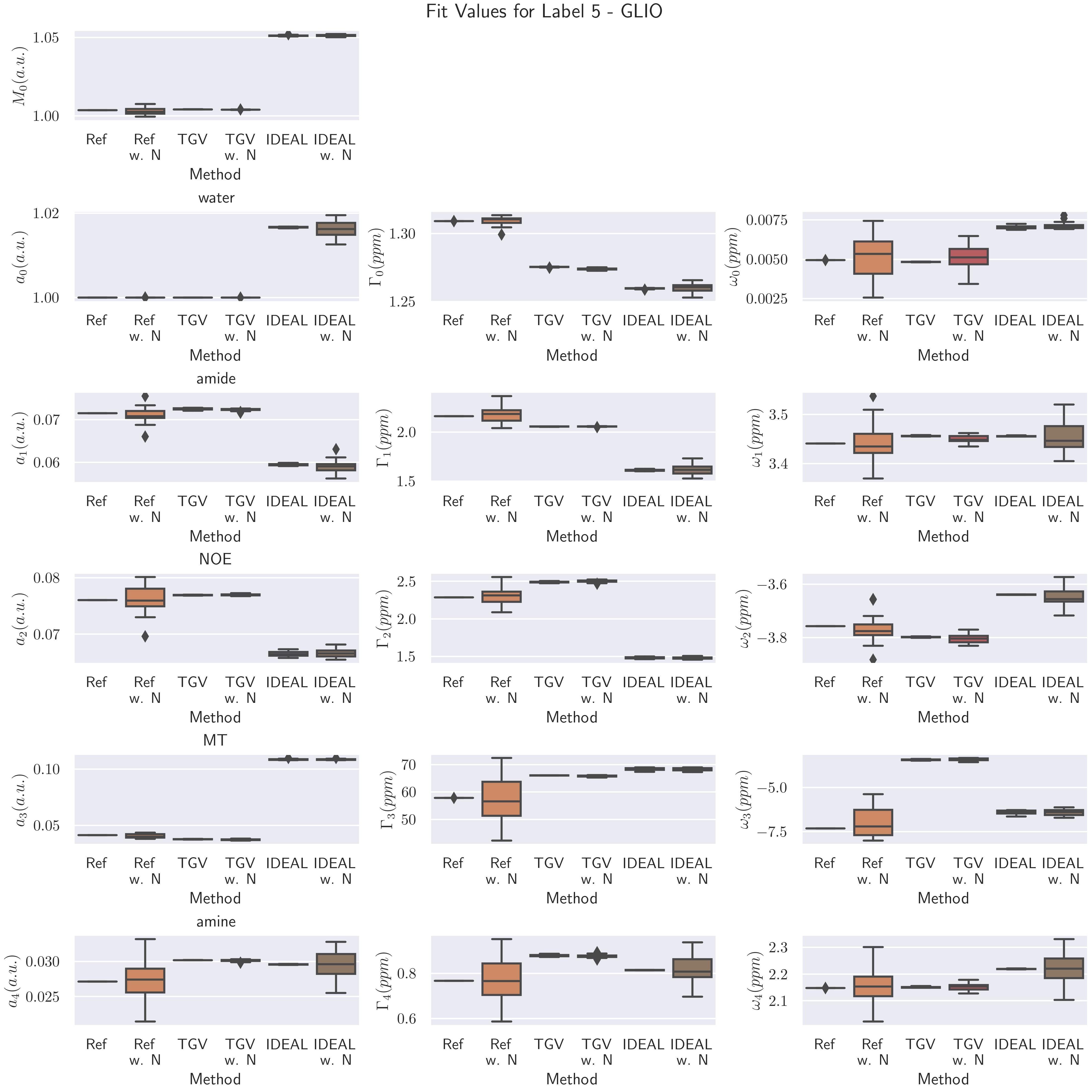
Figure 1 shows the resulting parameter maps for the numerical phantom for the reference, TGV fit and IDEAL fit. The tissue type is indicated in the label image. The $$$TGV_j$$$ regularized method results in lower noise for all parameter maps, while preserving sharp transitions between tissues. In $$$TGV_j$$$ and IDEAL, some parameter show a bias compared to the conventional reference fit (e.g. $$$M_0$$$, $$$a_1$$$, $$$a_1$$$, $$$\Gamma_1$$$, $$$\Gamma_2$$$, $$$\Gamma_4$$$). These needs to be investigated further, as a simultaneous change in line width and line amplitude must be related to the input parameters of solute concentration and solute exchange rate.In Figure 2, the parameter values in the simulated tissue 'Glioma' are depicted in box plots. All methods are shown with and without added noise. For this tissue, TGV-regularization significantly reduces noise, while the IDEAL implementation shows higher biases and lower noise reduction.
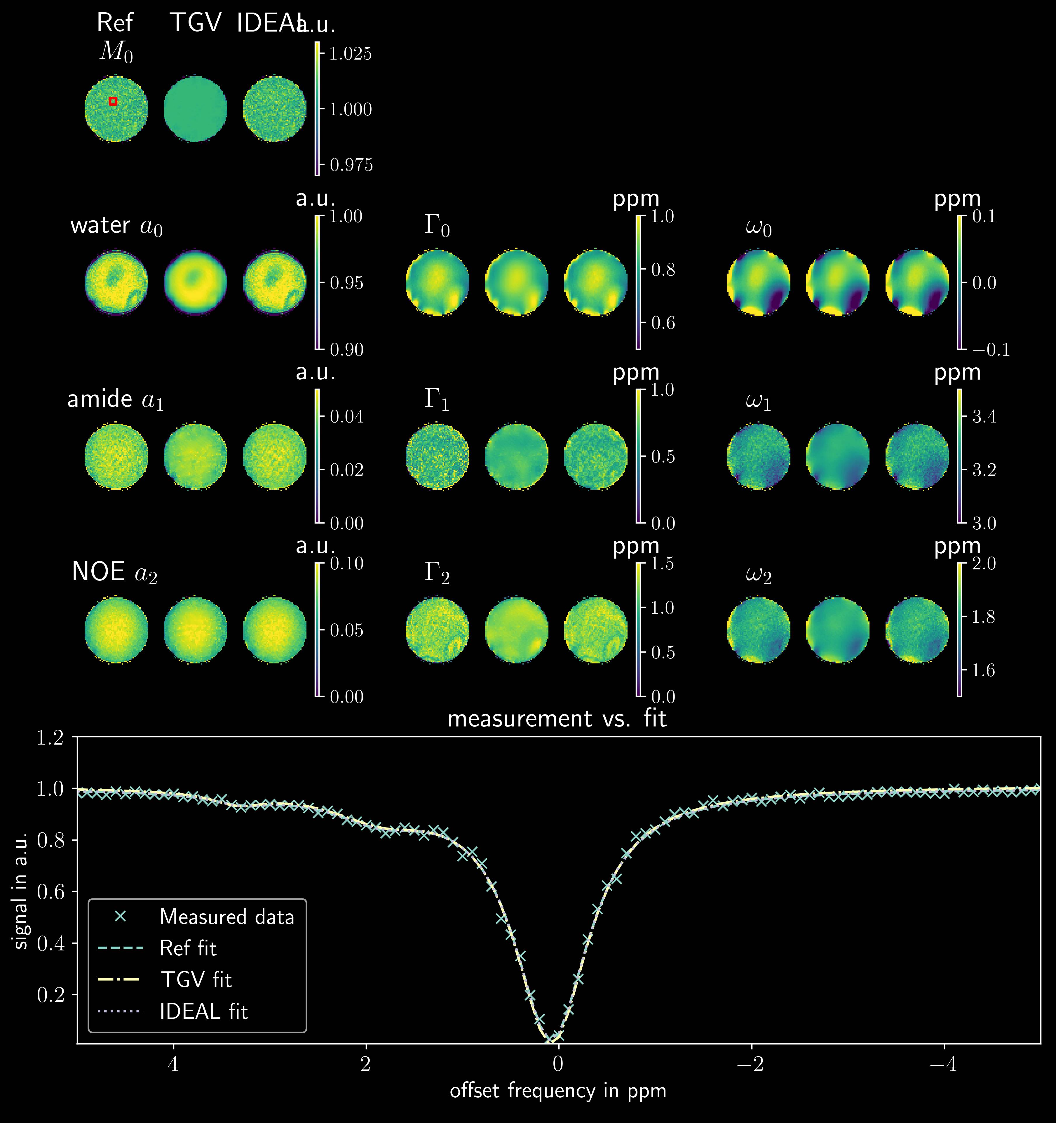
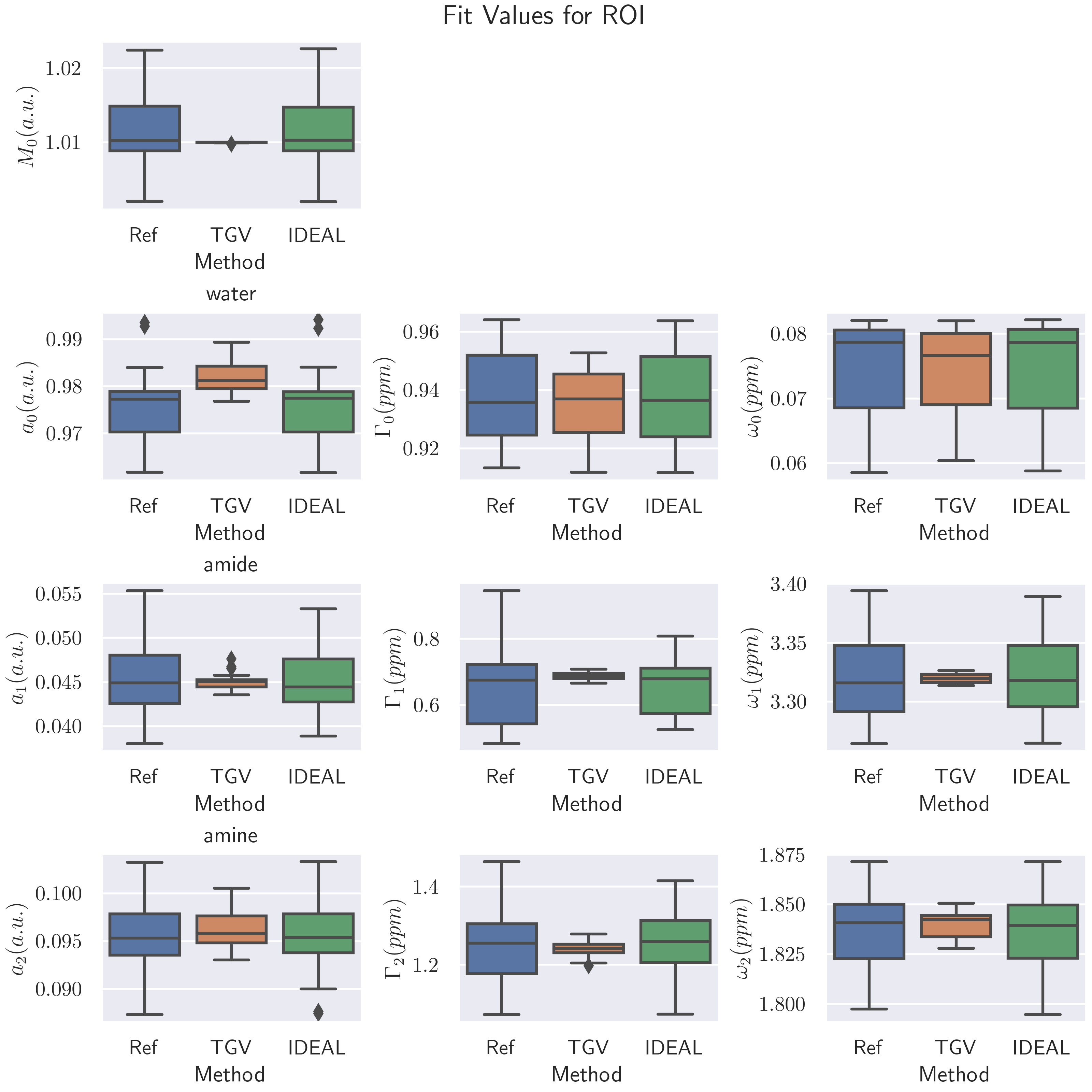
Figure 3 shows the parameter maps for the measured three pool phantom, while Figure 4 shows the parameters inside the ROI marked in red in Figure 3 as boxplots. As in the simulated data sets the joint spatial regularization approach outperforms the pixelwise fit and the IDEAL implementation in parameter map SNR. Figure 5 shows an example slice for a tumor patient. The TGV-method shows reduced noise, especially for the width parameters. The Goodness-of-Fit was determined for all scenarios, but showed very similar values for all three methods and could not explain the visible differences.
Conclusion
The proposed fitting method using joint spatial regularization shows improved stability and reduced noise using a three pool and five pool model for simulated and measured data. The reference method and the implemented IDEAL algorithm were outperformed in fitting stability and parameter map SNR.Acknowledgements
This research was funded in whole, or in part, by the Austrian Science Fund FWF-I4870 and by DFG ZA 814/5-1.References
1 M. Zaiß, et al., “Quantitative separation of CEST effect from magnetization transfer and spillover effects by Lorentzian-line-fit analysis of z-spectra”, J. Magn. Reson., vol. 211, no. 2, pp. 149–155, Aug. 2011, doi: 10.1016/j.jmr.2011.05.001.
2 O. Maier, et al., “Robust Lorentzian fitting of CEST spectra utilizing joint spatial regularization”, in Proceedings 30. Annual Meeting International Society for Magnetic Resonance in Medicine, 2022, vol. 30, p. 2079.
3 I. Y. Zhou, et al., “Quantitative chemical exchange saturation transfer (CEST) MRI of glioma using Image Downsampling Expedited Adaptive Least-squares (IDEAL) fitting”, Sci. Reports 2017 71, vol. 7, no. 1, pp. 1–10, Mar. 2017, doi: 10.1038/s41598-017-00167-y.
4 Bredies K, et al.,"Total generalized variation.", SIAM Journal on Imaging Sciences 3.3 (Jan. 2010), pp. 492-526. doi: 10.1137/090769521.
5 Bredies K, "Recovering Piecewise Smooth Multichannel Images by Minimization of Convex Functionals with Total Generalized Variation Penalty", Lecture Notes in Computer Science, 8293:44-77, 2014
6 F. Liu, et al.,"Fast Realistic MRI Simulations Based on Generalized Multi-Pool Exchange Tissue Model.", IEEE Transactions on Medical Imaging. 2016. doi: 10.1109/TMI.2016.2620961
7 K. Herz, et al., “Pulseq‐CEST: Towards multi‐site multi‐vendor compatibility and reproducibility of CEST experiments using an open‐source sequence standard”, Magn. Reson. Med., vol. 86, no. 4, pp. 1845–1858, Oct. 2021, doi: 10.1002/mrm.28825.
8 Liebert A, et al., "Multiple interleaved mode saturation (MIMOSA) for B1+ inhomogeneity mitigation in chemical exchange saturation transfer", Magn Reson Med. 2019 Aug;82(2):693-705. doi: 10.1002/mrm.27762.
9 Zaiss M, et al.,"Snapshot-CEST: Optimizing spiral-centric-reordered gradient echo acquisition for fast and robust 3D CEST MRI at 9.4 T.", NMR in Biomedicine 2018;31:e3879 doi: 10.1002/nbm.3879
10 Maier O, et al., "PyQMRI: An accelerated Python based Quantitative MRI toolbox", Journal of Open Source Software 5.56 (Dec. 2020), p. 2727. doi: 10.21105/joss.02727.
11 Chambolle A and Pock T. "A first-order primal-dual algorithm for convex problems with applications to imaging.", Journal of Mathematical Imaging and Vision 40.1 (2011), pp. 120-145. doi: 10.1007/s10851-010-0251-1.
Figures