3433
MRS Quantification using Deep Learning Frameworks: an Accuracy and Efficiency Study1Support Center for Advanced Neuroimaging (SCAN), University of Bern, Bern, Switzerland, 2Support Center for Advanced Neuroimaging (SCAN), Institute of Diagnostic and Interventional Neuroradiology, Bern, Switzerland
Synopsis
Keywords: Data Processing, Spectroscopy, Deep learning frameworks, Deep learning, Optimization
We implemented a model fitting algorithm for magnetic resonance spectroscopy quantification using Pytorch. This network fit the spectra by minimizing the error between the spectrum modeled by the newtwork and the desired target. The implementation can fit multiple spectras in parallel using Pytorch GPU acceleration. We compared the results with a parallel version of TDFDFit and found it to be up to 12 time faster fitting 2048 spectras in 50 seconds.Introduction
In vivo Magnetic Resonance Spectroscopy (MRS) can measure the chemical composition of tissues in a non-invasive way and allows the differentiation of brain-pathologies based on the concentration of specific metabolites. In the post-processing MRS-data, metabolite quantification is one of the most important steps since it allows the creation of quantitative maps of the brain. These quantifications are typically performed using nonlinear-least-squares (NLLS) fitting algorithms. Classical NLLS-methods have often low time-efficiency leading to long post-processing times, which makes high-spatially-resolve MRSI unattractive for use in clinical-routine. Reciently, deep-learning has proven useful for rapid quantification1,2, however, these methods are not yet robust, and incorrect training can lead to bias and low reliability3.In this work, we propose an NLLS-fitting implementation using Pytorch4 (DL-framework). This implementation works on GPU and TPU. It can fit any prior-knowledge-based model, which can simply be created with SpectrIm. We compare the performance of the proposed method with TDFDFit5 in terms of time-efficiency and accuracy of the results.
Methods
Prior Knowledge Model:The model we use to quantify the metabolites (as well as to simulate the spectra) is a linear combination model similar to the one used in LCModel6 and TDFDFit, represented as:
$$S(\omega)=FFT(e^{-W_c\,t\,+\,i\,(f_c\,t\,+\,\phi_c)}\sum_m\,A_m\,B_m(t)\,e^{-\Delta W_m\,t\,+\,i\,(\Delta f_m\,t\,+\,\Delta\,\phi_m)}) $$
where $$$A_m$$$ is a parameter related to the concentration for each metabolite, $$$W_c$$$, $$$\phi_c$$$ and $$$f_c$$$ are the common width, phase, and frequency shift respectively and $$$B_m(t)$$$ is the normalized time-domain basis set. Here the parameters $$$\Delta\,W_m=(W_m-W_c)$$$, $$$\Delta\,\phi_m=(\phi_m-\phi_c)$$$ and $$$ \Delta\,f_m=(f_m-f_c)$$$ are the prior-knowledge fixed parameters defined in the model. In this approach, the quantification of M spectral components reduces from a 4M-dimentional to a M+3-dimensional NLLS-problem, which reduces the Cramér-Rao-minimum-variance-bound (CR-MVB).
Simulated dataset:
We simulated a dataset of spectra of a model consisting of 15 metabolites. The model was developed to quantify ultra-high-field (7T) SLOW-EPSI-data. Each metabolite basis-element was simulated using NMRScope-B7. The area parameters of all components were varied in a range of 0.1 and 2.0 times the initial parameters-values of the model, defined such that the model fit the average spectra on clinical cases. We added Gaussian noise to the generated dataset to study quantification performance as a function of the signal-to-noise-ratio (SNR). Each SNR-dataset consisted of 2048 spectra.
Fitting strategy:
The Pytorch fitting strategy consists of the following steps:
1) Find the initial frequency-shifts for each spectrum by maximizing the cross-correlation between the initial-value spectrum and the target spectrum. This approach reduces the likeliness of ending up in a local-minima.
2) Generate the target of the fit by concatenating a set of N simulated spectra. This approach enables the Pytorch-model to fit multiple spectra in parallel.
3) Fit by backpropagating the Pytorch-model and updating the parameters (trainable tensors) until the convergence of the so-called MeanSquaredError between the target and the output of the network is reached. Normalization was performed with respect to the noise-level. This forces the loss to ignore the amount of noise. Figure 1 shows the pipeline corresponding to above-described steps.
Hyperparameters were lr=1, optmimizer=Adam, epoch_number=3000, patience=40, and device=cuda for all the performed fittings. As convergence criteria, a loss improvement of less than 0.001% was chosen.
Results
Since there is no ground-truth for the parameters obtained from clinical cases, we tested only on simulated datasets, and compare them with TDFDFit. In the past TDFDFit has been multiple times compared with LCModel (regarded by many colleagues as standard). No significant differences were observed8 between both methods. The SNR was varied in the range between 50 and 5 to study the performance under more realistic conditions.In Figure 2 we show the time-efficiency of our algorithm running on an NVIDIA-GTX-1060-6GB, compared to a CPU-based parallelized version of TDFDFit (AMD-Ryzen 7-2700X, 16threads). We obtain an average of 11x-acceleration, increasing to even 12 for low SNR spectra. As expected, for a small number of spectra, there is no advantage of GPU use. In our case of interest (EPSI-datasets) approximately 20000 spectra must be quantified: in this case, a speed-up from 1:30 Hs to 8.5 minutes is expected.
In Table 1 we present the percentual error for each parameter in the model and every SNR-value in contrast to the error obtained using TDFDFit. The optimal performance is demarcated In bold.
Figure 3 shows the scatter and correlation between the ground-truth and both methods for the most important metabolites in this SLOW-EPSI model (GABA, Glx, 2-HG, NAA) for the case of SNR=10. No significant difference between both models is observed for the cases where the peak is appreciable in comparison to the noise. Table 1 shows the error for both methods. In accordance with the CR-MVB, weak metabolites cannot be differentiated from the background by either of the methods.
Finally, Figure 4 (a) shows an example of spectra fitted with both methods and (b) the fitting residual, again, there is no significant difference between both methods
Discussion
We presented a fitting strategy using Pytorch to solve the problem of metabolite-quantification by accelerated NLLS-fitting using GPUs and the advantages of Pytorch’s optimizers: fitting performance w.r.t. accuracy is equivalent to traditional fitting approaches as LCModel/TDFDFit.Furthermore, significant increases in processing speed of up to 12x is obtained using the Pytorch-based parallel optimization method using GPUs.
Acknowledgements
The project leading to this application has received funding from the European Union's Horizon 2020 research and innovation programme under the Marie Sklodowska-Curie grant agreement No 813120References
1) Gurbani, S. S., Sheriff, S., Maudsley, A. A., Shim, H., & Cooper, L. A. (2019). Incorporation of a spectral model in a convolutional neural network for accelerated spectral fitting. Magnetic resonance in medicine, 81(5), 3346-3357.
2) Hatami, N., Sdika, M., & Ratiney, H. (2018, September). Magnetic resonance spectroscopy quantification using deep learning. In International Conference on Medical Image Computing and Computer-Assisted Intervention (pp. 467-475). Springer, Cham.
3) Rizzo, R., Dziadosz, M., Kyathanahally, S.P., Reyes, M., Kreis, R. (2022). Reliability of Quantification Estimates in MR Spectroscopy: CNNs vs Traditional Model Fitting. In: Wang, L., Dou, Q., Fletcher, P.T., Speidel, S., Li, S. (eds) Medical Image Computing and Computer Assisted Intervention – MICCAI 2022. MICCAI 2022. Lecture Notes in Computer Science, vol 13438. Springer, Cham.
4) et al., 2019. PyTorch: An Imperative Style, High-Performance Deep Learning Library. In Advances in Neural Information Processing Systems 32. Curran Associates, Inc., pp.
5) Slotboom, J., Boesch, C., & Kreis, R. (1998). Versatile frequency domain fitting using time domain models and prior knowledge. Magnetic resonance in medicine, 39(6), 899-911.
6) Provencher SW. Estimation of metabolite concentrations from localized in vivo proton NMR spectra. Magn Reson Med 1993;30(6):672–679.
7) Starčuk Z Jr, Starčuková J. Quantum-mechanical simulations for in vivo MR spectroscopy: Principles and possibilities demonstrated with the program NMRScopeB. Anal Biochem. 2017; 15;529:79-97.
8) Hofmann, L., Slotboom, J., Jung, B., Maloca, P., Boesch, C. and Kreis, R., 2002. Quantitative 1H‐magnetic resonance spectroscopy of human brain: influence of composition and parameterization of the basis set in linear combination model‐fitting. Magnetic Resonance in Medicine: An Official Journal of the International Society for Magnetic Resonance in Medicine, 48(3), pp.440-453.
Figures
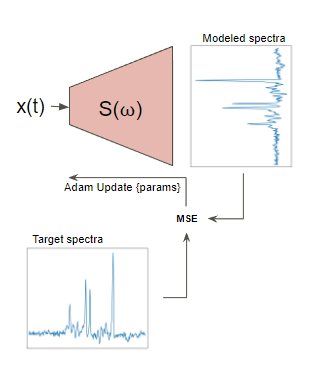
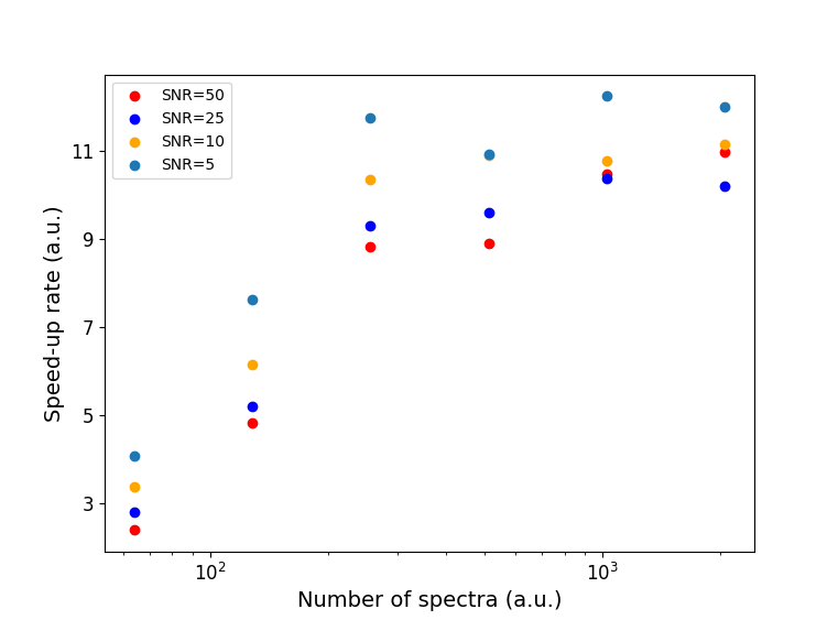
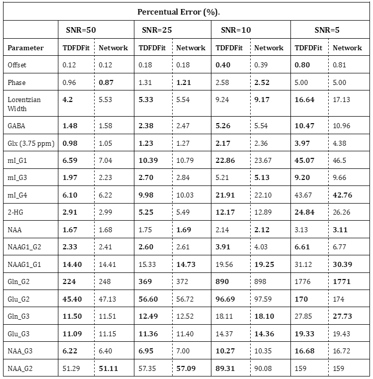
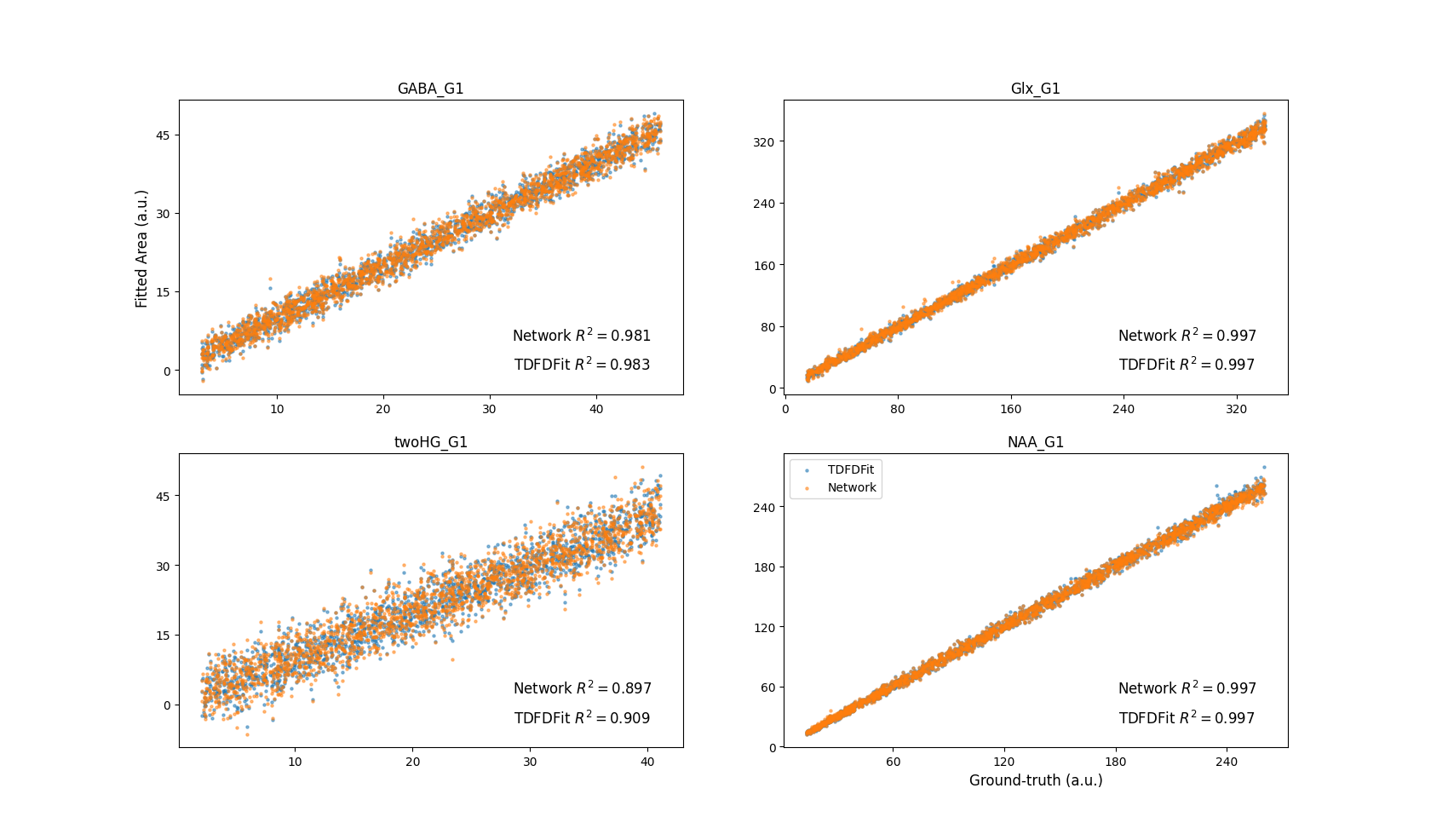
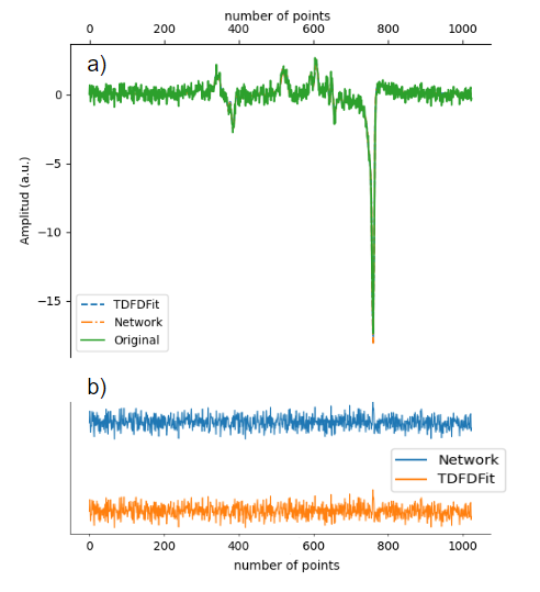
Figure 4: Example of Fitting using both methods, a) shows the original spectra with both dashed lines representing the best fit for each model. b) shows the residual of the fitting for TDFDFit (orange) and the Pytorch model (Blue).