Synopsis

Keywords: Artifacts, System Imperfections: Measurement & Correction, GIRF, GSTF, LTI

We compared three different trajectory correction methods in spiral phantom images on a preclinical 7T scanner with a high-performance gradient insert. The first was an isotropic delay-correction, the second a gradient correction based on the gradient system transfer function (GSTF), and the third employed measured trajectories. In both an axial and a double-oblique slice, the measured trajectory resulted in the best image quality, while the delay-corrected images suffered from halo effects and signal bleeding. The GSTF-corrected images only had minor remaining artifacts, stemming from trajectory deviations due to non-linearities in the gradient chain.

Introduction

Spiral k-space trajectories^1,2 have been used in an increasing number of clinical MRI applications in recent years^3–5. However, they have only been sparsely reported in preclinical research settings^6,7, which typically feature higher magnetic field strengths and stronger, faster switching gradient systems. Thus, the inherent sensitivity of spiral trajectories to off-resonance, field inhomogeneity, and gradient imperfections impose significant limitations, which have to be addressed adequately. Measuring the true gradient progression in a separate measurement⁸ is a common solution to avoid artifacts caused by gradient infidelities. Conversely, linear, time-invariant (LTI) characteristics of the gradient chain can be determined in the form of the gradient system transfer function (GSTF)⁹, which in turn can be used to predict the actual trajectories^10,11. In this study, we compare three different trajectory correction methods in spiral phantom images on a preclinical 7T scanner with a high-performance gradient insert.

Methods

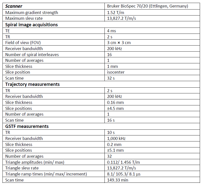
We acquired an axial and a double-oblique slice with the parameters given in Table 1. For image reconstruction, we used the non-uniform FFT (NUFFT) toolbox¹². We performed four image reconstructions, each using a different k-space trajectory: 1. the prescribed trajectory, 2. a delay-corrected trajectory, 3. a GSTF-predicted trajectory, 4. a measured trajectory. For the delay-corrected trajectory, the prescribed gradient progressions were delayed by 25 µs. This delay gave the lowest RMS error (0.008 a.u.) between the delay-corrected axial image and the one with the measured trajectory, which we considered as ground-truth. The measured trajectory was obtained with the thin-slice method proposed by Duyn et al.⁸ immediately before image acquisition. The GSTF was computed from the measured response to 13 triangular gradient pulses^9,13, which were also acquired with the thin-slice method⁸. With the GSTF, the expected gradient progressions were calculated in the frequency domain⁹ and the result in the time domain was numerically integrated to yield the predicted trajectory. The GSTF-correction incorporated an additional delay-correction of -40 µs to account for non-linear effects in the gradient chain¹⁴. This delay was also determined by minimizing the RMS error (0.006 a.u.) to the ground-truth axial image.

Results

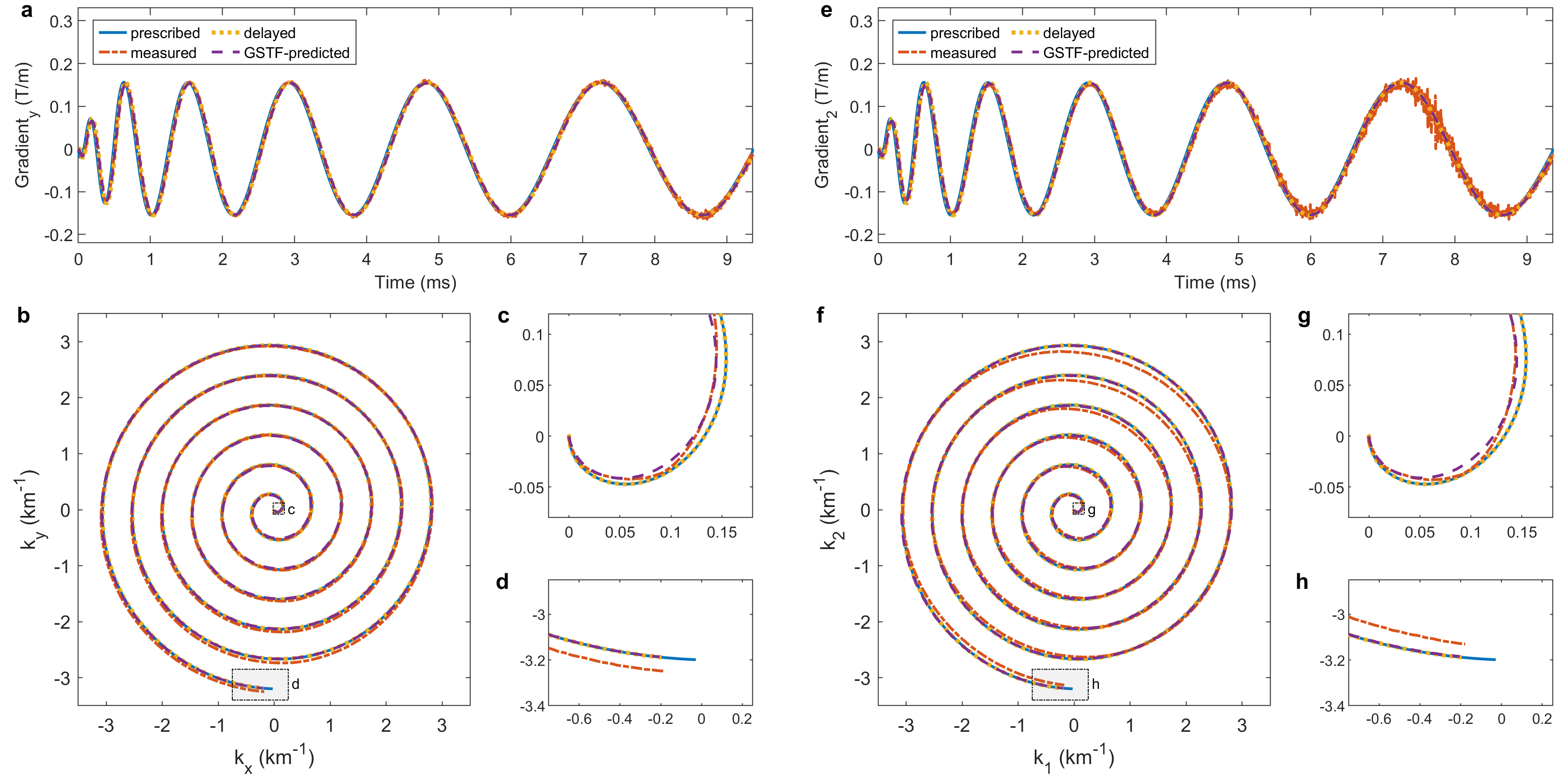
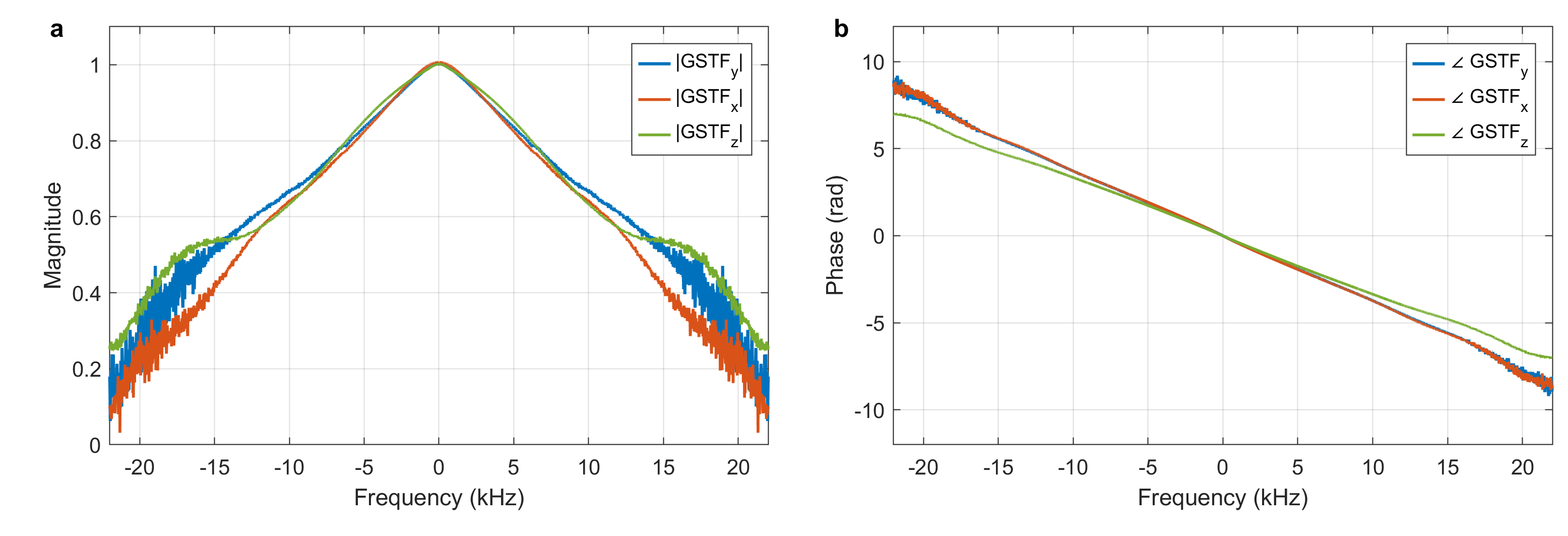
Figure 1 (a-d) show the gradient progressions of one of the 16 spiral arms on the y-axis (a) and the corresponding k-space trajectories (b-d) for the axial image acquisition. In (e-h), the corresponding curves for the double-oblique image are shown. Each subplot contains four lines, corresponding to the prescribed, delay-corrected, GSTF-corrected, and measured trajectory. In the k-space center ((c) and (g)), the GSTF-corrected trajectory agrees well with the measured one, whereas in the k-space periphery, it rather coincides with the delay-corrected trajectory ((d) and (h)). Both the prescribed and the delay-corrected trajectory exhibit distinct deviations from the measured trajectory over their whole course.
Figure 2 displays the GSTF self-terms of the x-, y- and z-axis.
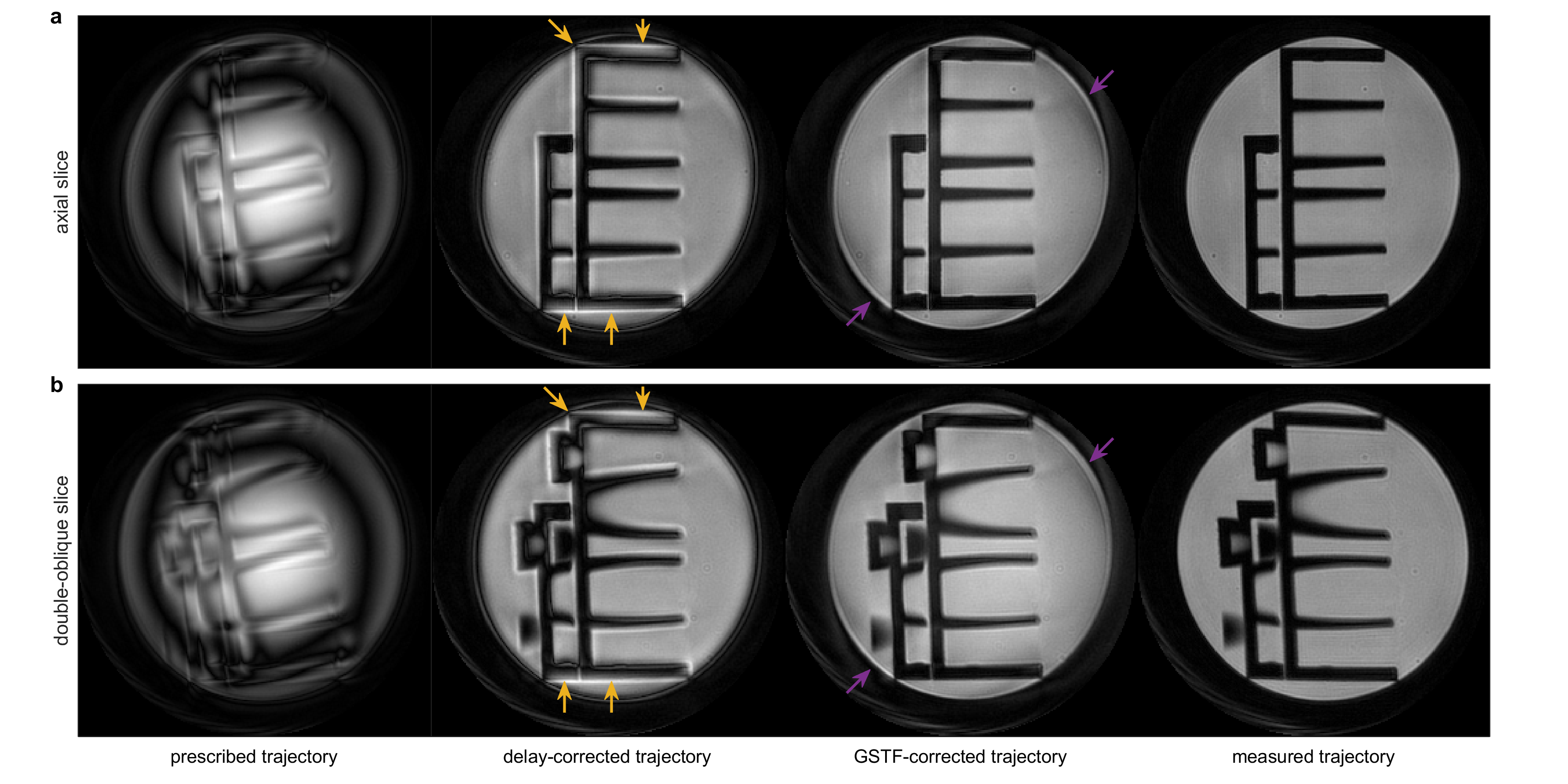
The reconstructed images are presented in Figure 3.

Discussion

In Figure 3, we can see a successive improvement in image quality from left to right. The images reconstructed with the prescribed trajectory suffer from heavy artifacts such as blurring and intensity variations. With the delay-correction, the structure of the phantom appears more clearly, but still shows significant halo effects at the edges and signal bleeding into dark areas towards the outer portions of the FOV (marked by yellow arrows). The GSTF-correction almost eliminates both of these issues. The most noticeable remaining artifact is a slight overemphasis of the phantom’s rim (marked by violet arrows). Furthermore, the signal intensity looks less uniform across the image compared to the reconstructions with the measured trajectories, which appear artifact-free.
The differences between the images are a result of the discrepancies between the k-space trajectories, which are revealed in Figure 1. The pure delay-correction ignores the low-pass transmission behavior of the gradient chain, which is reflected in the magnitude of the GSTF (Figure 2(a)). The GSTF, on the other hand, only accurately characterizes linear, time-invariant features of the gradient system. Violations of these assumptions¹⁴ cause deviations of the GSTF-predicted from the measured trajectory.
However, the GSTF-correction yields superior image quality compared to the delay-correction, and is thus a powerful tool for applications, in which a separate trajectory measurement is not feasible. This may, for example, be the case when timing restrictions apply, or very high gradient amplitudes are employed, or the sample is very small or has a very short T2*. The thin-slice method relies on the phase evolution of the FID signal, which can only be extracted confidently if the signal magnitude is not too low. This makes measuring gradients with high amplitudes or over long time-periods generally challenging with this technique. In Figure 1(a) and (e), the measured gradient progressions already show increased noise towards the end of the readout, even though we only measured in a phantom, and not in vivo. The GSTF-based trajectory correction avoids these issues.

Conclusion

We compared different trajectory correction methods for spiral imaging on a preclinical MRI scanner. While a separate measurement of the trajectory enabled the best image quality, the GSTF-correction produced almost artifact-free images, clearly improving over a pure isotropic delay-correction.

Acknowledgements

No acknowledgement found.

References

1. Ahn CB, Kim JH, Cho ZH. High-Speed Spiral-Scan Echo Planar NMR Imaging-I. IEEE Trans Med Imaging. 1986;5(1):2-7. doi:10.1109/TMI.1986.4307732

2. Meyer CH, Hu BS, Nishimura DG, Macovski A. Fast Spiral Coronary Artery Imaging. Magn Reson Med. 1992;28(2):202-213. doi:10.1002/mrm.1910280204

3. Glover GH. Spiral imaging in fMRI. NeuroImage. 2012;62(2):706-712. doi:10.1016/j.neuroimage.2011.10.039

4. Lee Y, Wilm BJ, Brunner DO, et al. On the signal-to-noise ratio benefit of spiral acquisition in diffusion MRI. Magn Reson Med. 2021;85(4):1924-1937. doi:10.1002/mrm.28554

5. Eirich P, Wech T, Heidenreich JF, et al. Cardiac real-time MRI using a pre-emphasized spiral acquisition based on the gradient system transfer function. Magn Reson Med. 2021;85(5):2747-2760. doi:10.1002/MRM.28621

6. Zhong X, Gibberman LB, Spottiswoode BS, et al. Comprehensive Cardiovascular magnetic resonance of myocardial mechanics in mice using three-dimensional cine DENSE. J Cardiovasc Magn Reson. 2011;13(1):83. doi:10.1186/1532-429X-13-83

7. Castets CR, Lefrançois W, Wecker D, et al. Fast 3D ultrashort echo‐time spiral projection imaging using golden‐angle: A flexible protocol for in vivo mouse imaging at high magnetic field. Magn Reson Med. 2017;77(5):1831-1840. doi:10.1002/mrm.26263

8. Duyn JH, Yang Y, Frank JA, van der Veen JW. Simple Correction Method fork-Space Trajectory Deviations in MRI. J Magn Reson. 1998;132(1):150-153. doi:10.1006/jmre.1998.1396

9. Vannesjo SJ, Haeberlin M, Kasper L, et al. Gradient system characterization by impulse response measurements with a dynamic field camera. Magn Reson Med. 2013;69(2):583-593. doi:10.1002/mrm.24263

10. Addy NO, Wu HH, Nishimura DG. Simple method for MR gradient system characterization and k-space trajectory estimation. Magn Reson Med. 2012;68(1):120-129. doi:10.1002/mrm.23217

11. Campbell-Washburn AE, Xue H, Lederman RJ, Faranesh AZ, Hansen MS. Real-time distortion correction of spiral and echo planar images using the gradient system impulse response function. Magn Reson Med. 2016;75(6):2278-2285. doi:10.1002/mrm.25788

12. Fessler JA, Sutton BP. Nonuniform fast Fourier transforms using min-max interpolation. IEEE Trans Signal Process. 2003;51(2):560-574. doi:10.1109/TSP.2002.807005

13. Wilm BJ, Dietrich BE, Reber J, Johanna Vannesjo S, Pruessmann KP. Gradient Response Harvesting for Continuous System Characterization during MR Sequences. IEEE Trans Med Imaging. 2020;39(3):806-815. doi:10.1109/TMI.2019.2936107

14. Brodsky EK, Samsonov AA, Block WF. Characterizing and correcting gradient errors in non-cartesian imaging: Are gradient errors linear time-invariant (LTI)? Magn Reson Med. 2009;62(6):1466-1476. doi:10.1002/mrm.22100