3420
Spatiotemporal B0 correction in Oscillating Steady State Imaging (OSSI) fMRI using Free Induction Decay Navigators (FIDnavs)1Biomedical Engineering, University of Michigan, Ann Arbor, MI, United States, 2Electrical Engineering, University of Michigan, Ann Arbor, MI, United States, 3Hyperfine Research, Guilford, CT, United States
Synopsis
Keywords: Artifacts, Shims, B0 correction
Temporal field variations (e.g., physiological noise) in oscillating steady state imaging (OSSI) not only increases signal fluctuations as seen in GRE, but also alters signal characteristics that lead to inconsistent k-space acquisitions from TR to TR. This effectively reduces the overall functional contrast and temporal signal to noise ratio (tSNR). Here, we utilized free induction decay (FID) signal phase to estimate up to the first-order field inhomogeneity coefficients for prospective spatiotemporal B0 field correction in OSSI.Introduction
Oscillating steady state imaging (OSSI) is a steady state sequence that utilizes quadratic RF phase increments with balanced gradients to produce a high SNR $$$T_{2}^{*}$$$ weighted signal that oscillates with a periodicity of $$$n_c\times TR$$$1, where $$$n_c$$$ is the number of RF phase cycles used ($$$\sim$$$6-10). OSSI phase cycled images exhibit large B0-dependent banding due to the oscillations, and these can be averaged out by combining across $$$n_c$$$ to produce a more uniform signal. OSSI is highly sensitive to off-resonance, which is leveraged to detect the BOLD changes needed for fMRI studies, however, OSSI also has increased susceptibility to B0 off-resonance artifacts from respiration and field drifts. The phase of the OSSI signal varies non-linearly with off-resonance leading to a complex time-varying response to respiration. Therefore conventional GRE-based correction methods have proven ineffective for OSSI2. We have previously utilized the Free induction decay (FID) phase navigators3 to measure B0 inhomogeneity and performed zeroth-order compensation in real-time4. Zeroth-order correction is insufficient for non-axial slices or 3D acquisition, however rapid B0 shimming can be used to perform higher-order correction since shim settings can be rapidly updated by changing individual shim currents. Here, we demonstrated a method of using OSSI FID phase to estimate constant and linear shim inhomogeneity coefficients based only on the sensitivity differences across a multicoil receiver array.Methods
Our approach first involves a calibration stage, where the response of each shim coil to a given input offset is characterized for each receive coil in the array. The process is given by:$$\begin{bmatrix} a_{0,1} & \dots & a_{0,n}\\ a_{x,1} & \dots & a_{x,n}\\ a_{y,1} & \dots & a_{y,n} \\\end{bmatrix} = T\begin{bmatrix} m_{11} & \dots & m_{1k}\\ \vdots & \dots & \vdots \\ m_{n1} & \dots & m_{nk} \\\end{bmatrix} \ \ \ (1)$$ where $$$A$$$ is a $$$3 \times n$$$ matrix of applied offsets for $$$n$$$ calibrations of the zeroth and first order shims ($$$\Delta f$$$, $$$x$$$, and $$$y$$$). $$$M$$$is a $$$n \times k$$$ matrix of relative FID phases corresponding to the different calibrations, $$$n$$$, for each coil element, $$$k$$$. $$$T_{ik}$$$ is a $$$3 \times k$$$ calibration matrix which describes the amount of field $$$i$$$ generated by the $$$k_{th}$$$ receive coil. Given $$$A$$$ and $$$M$$$, $$$T$$$ can be estimated by solving the inverse problem posed in equation1.Shim coefficients can then be dynamically estimated using: $$a_t = Tm_t \ \ \ (2) $$ where $$$m_t$$$ is a $$$k \times 1$$$ vector of FID phase changes for each coil at timepoint, t.
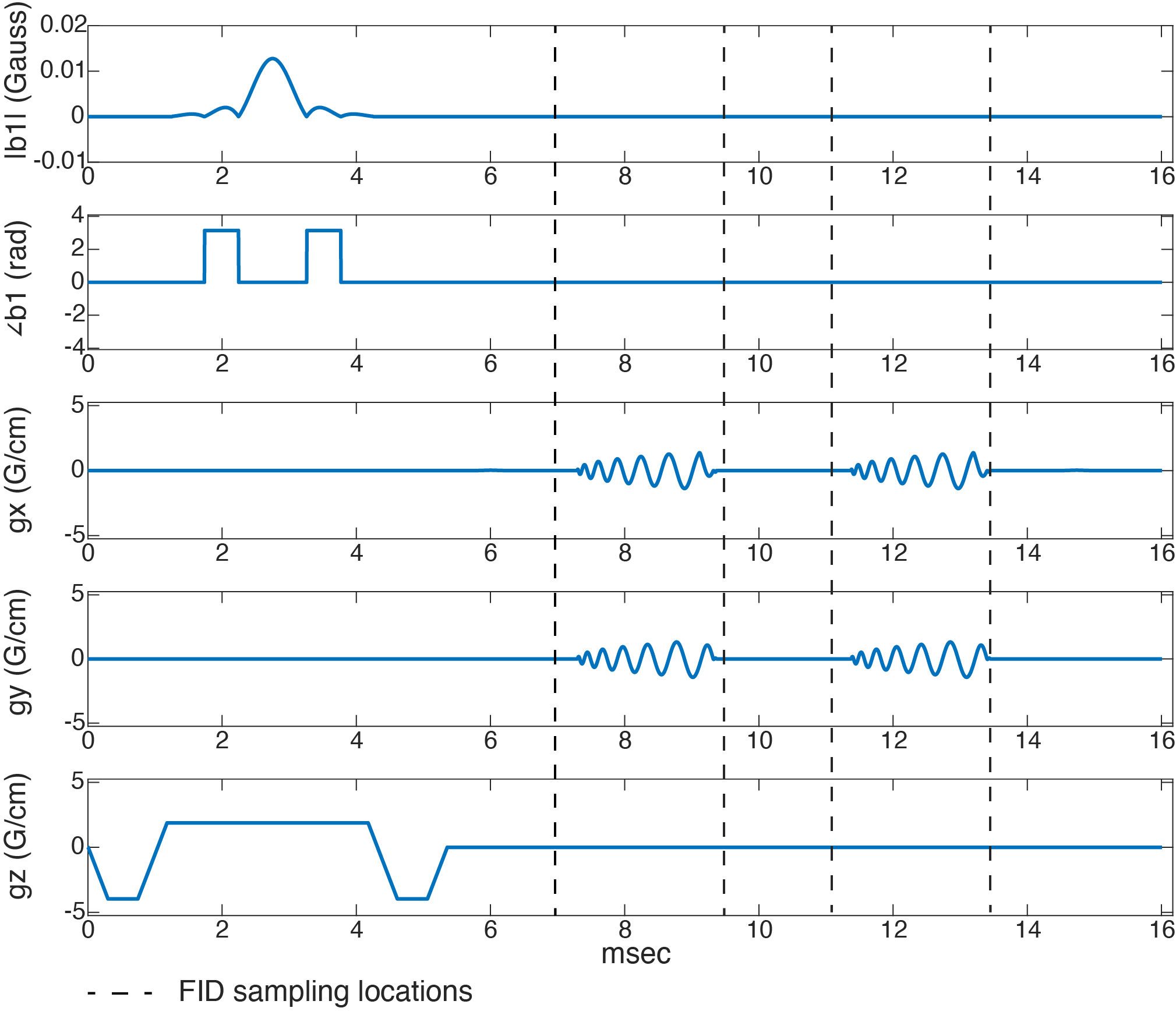
Data Acquisition:This technique was evaluated for an axial slice with a double echo readout using a single-shot balanced variable density spiral-out trajectory (Fig. 1). An additional 1ms long FID was placed before and after each spiral readout.The scan was acquired with TR=16ms, nc=10, effective TR = 160ms, FOV=24cm, pixel size=25x25cm, $$$\Delta $$$TEfid=3.1ms, $$$\Delta$$$TEspirals=4.1ms and FA=10$$$^{\circ}$$$.
We performed an fMRI experiment with a functional task of finger-tapping, where subjects were asked to tap their fingers for 20s and rest for 20s, repeated 5 times (scan duration 200s), in order to provide realistic fMRI data with activations to test the $$$B_0$$$ tracking. The scan was repeated three times with normal breathing, deep breathing, and rotating and tilting their head slightly
Navigator Calibration:FID signals were acquired with the $$$x$$$ and $$$y$$$ shim coils at multiple current offsets. We specifically added a +/-100Hz offset across the FOV which corresponds to 0.02G/cm gradient amplitude. The FID phase changes induced by the shim offsets were then subtracted from a reference FID phase acquired without any shim offsets. Equation 1 was then used to generate the calibration matrix $$$T$$$. This is performed once for each subject.
Estimating First-order shim inhomogeneity Coefficient: Field changes were estimated from the FID signal by computing the phase difference between the FIDs sampled before and after the spiral readout. 0.2ms of the FID signals were discarded to avoid filter transients. Equation 2 was then solved to estimate up to the first order shim inhomogeneity coefficients. Conventional fieldmaps were generated from OSSI images reconstructed from the two spiral readouts. We directly fitted the linear basis to the field map for comparison to our FID-based approach.
Results
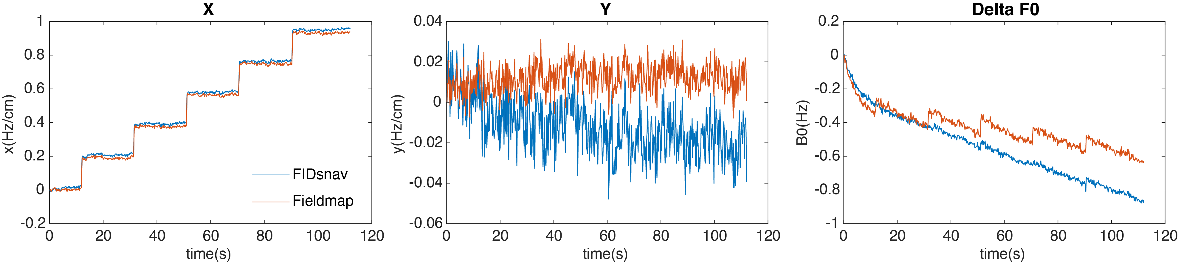
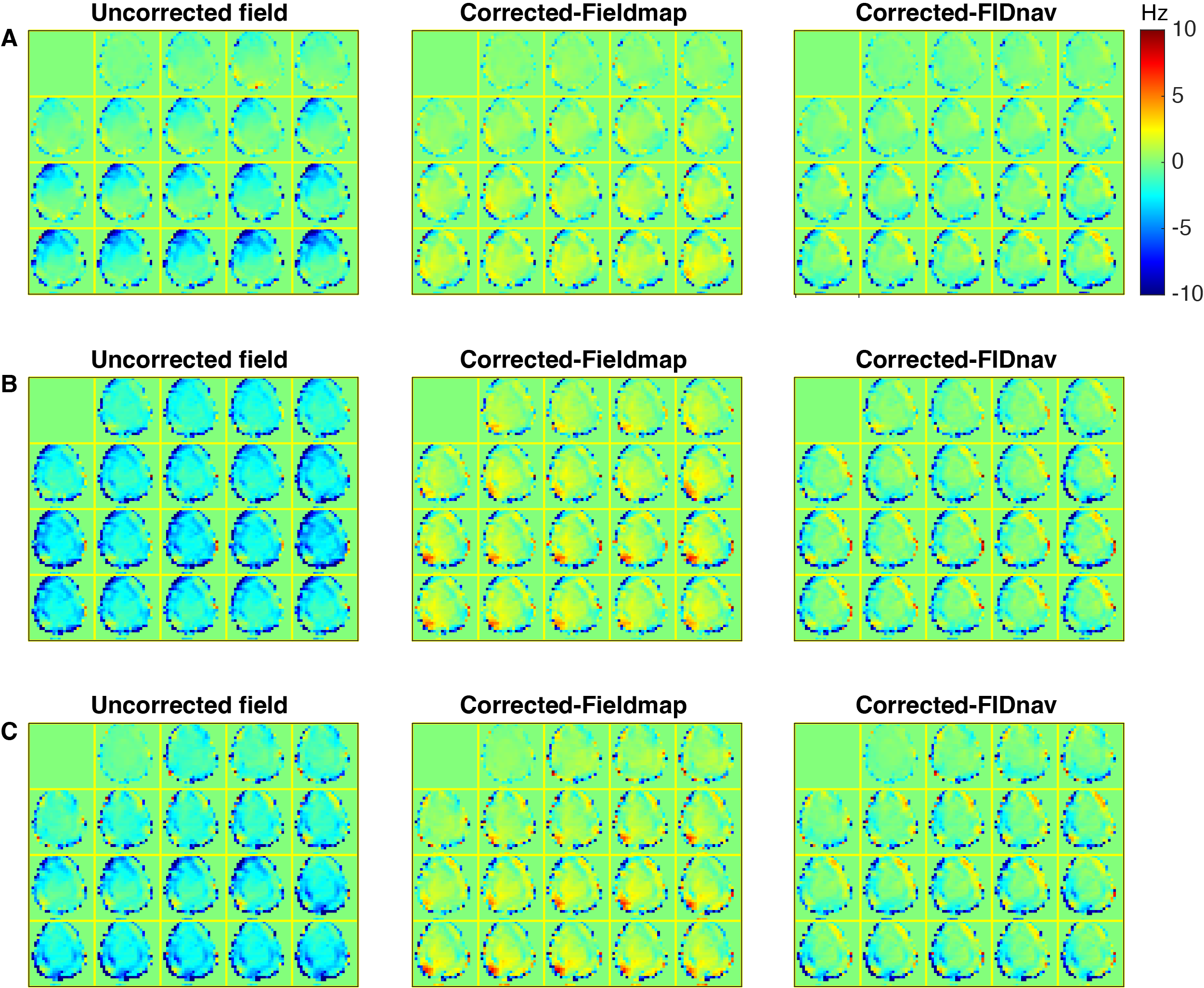
Phantom results show good level of agreement between coefficients from FIDnav and the fieldmap as seen in Fig.2.In-vivo results in Fig.3 show that corrections based on FIDnavs significantly reduced respiration and motion induced field changes, thereby making field changes from subsequent TRs more consistent with the first TR compared to the uncorrected field.
Moreover, the frequency timecourses in Fig.4 show less fluctuations for all three experimental conditions in FIDnav correction with small residuals compared to the uncorrected timecourse.
Discussion & Conclusion
In this study we estimated first order field inhomogeneity coefficients during an OSSI fMRI experiment based on FID signals sampled at the center of a spiral-out kspace for a 32-channel array. Our preliminary experiments show promising results for normal breathing, deep breathing, and motion in axial slices. In the future, we plan to characterize and correct the effects of eddy currents for spiral rotations and also apply the FIDnav to prospectively correct OSSI images. So far, we have only applied this method in axial slices, our next step will be to test performance in sagittal slices and 3D imaging.Acknowledgements
We wish to acknowledge the support of NIH Grants U01EB026977 & F32EB029289.References
[1] Shouchang Guo and Douglas C Noll. Oscillating steady-state imaging (ossi): A novel method for functional mri. Magnetic Resonance in Medicine,84(2):698–712, 2020.
[2] Amos A Cao and Douglas C Noll. A retrospective physiological noise correction method for oscillating steady-state imaging. Magnetic Resonance inMedicine, 85(2):936–944, 2020.
[3] Tess E Wallace, Onur Afacan, Tobias Kober, and Simon K Warfield. Rapid measurement and correction of spatiotemporal B0 field changes using fid navigators and a multi-channel reference image. Magnetic resonance inmedicine, 83(2):575–589, 2020.
[4] Amos A Cao and Douglas C Noll. Real-time respiration compensation inoscillating steady state fmri. In Proceedings of the annual meeting of the ISMRM, Virtual Conference,2020,Abstract 1223.
Figures
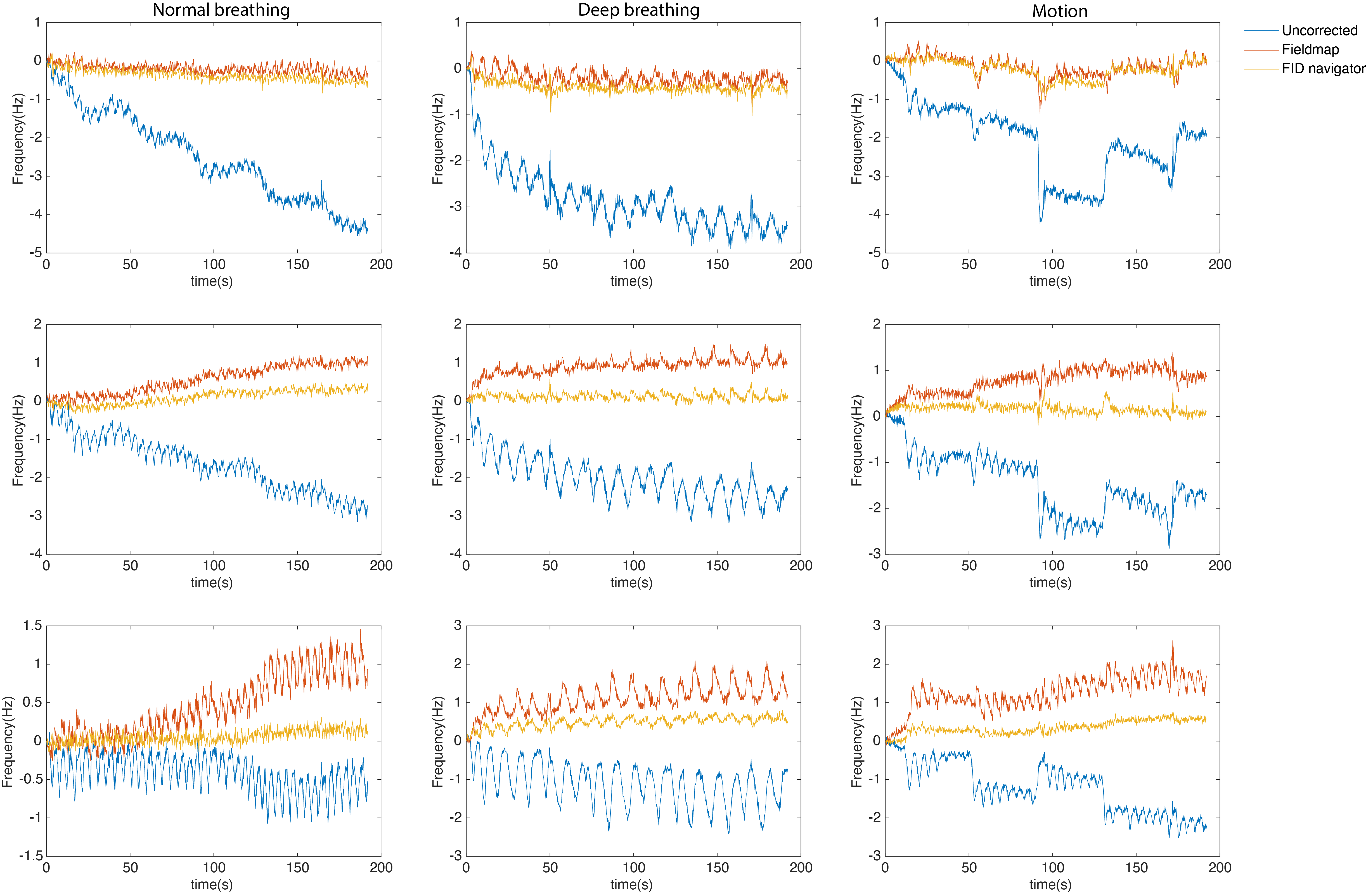
Frequency timecourses with B0 correction based on the fieldmap and FIDnav compared to the uncorrected field in normal breathing, deep breathing, and motion. This was done for three voxels (top two rows: active voxels, and bottom row: non-active voxel.