Synopsis

Keywords: System Imperfections: Measurement & Correction, Simulations

In this work, we derived an equation describing the signal evolution during an SGRE sequence with preparation pulses. The signal changes especially during the earlier RF pulses and differs from the values for later RF pulses, where it approaches the signal from an SPGR sequence without prepulses. Using the derived equation might enable more accurate DCE examinations.

Introduction

Abdominal aortic aneurysm (AAA) is a degenerative inflammatory disease of the aortic wall which when getting ruptured becomes life-threatening. AAA progression may be assessed using dynamic contrast-enhancement (DCE) MRI¹. Imaging the vessel walls of AAA patients requires suppression of blood and fat signal to accurately image the contrast uptake. However, the usage of blood and fat suppression disrupts the steady state of the spoiled gradient echo (SGRE), which is generally used to acquire DCE MRI. Therefore, conventional approaches to convert signal into contrast concentration may be inadequate. Hence, to investigate the effect of black blood and fat suppression prepulses on the signal, we modelled the signal evolution for an SGRE combined with preparation prepulses and validated it in a phantom with known T1 properties.

Methods

Theory
A GRE with fat suppression and black blood typically consists of a block of N (Turbo Field Factor) regular GRE pulses, interleaved with a block with a SAR and fat suppression block (to apply fat suppression and limit SAR), a black blood block² and an additional spoiling block (Fig.1). During the fat suppression and spoiling blocks, the spins of interest undergo T1 relaxation, whereas during the black blood block, the spins of interest undergo T2 relaxation as they are in the x-y plane. To accommodate for this additional T1 and T2 relaxation, we extended the formula of a conventional SGRE to include these pre-pulses.
The longitudinal magnetization available before each of the N RF-pulses within a shot is given by:

$$ M_n^-=M_0 (1-E_1 )*\frac{1-[E_1*cos⁡(α) ]^n}{1-E_1*cos⁡(α) }+M_0^-*cos^n⁡(α)*E_1^n $$

Where n is the number of the RF pulses starting from 0 until N-1, N is the total number of RF pulses within one shot and is the longitudinal magnetization at the end of the preparation just before the first RF pulse ($$$\alpha$$$ is the flip angle and $$$M_0$$$ the net magnetization in z-direction; See Fig.1). Instead of having a steady-state during each RF pulse, the steady-state will repeat itself during each block of RF pulses^3,4, which leads to $$$M_0^-$$$:

$$ M_0^-=((M_N^-*E_{Fat-sat}+M_0 (1-E_{Fat-sat}))*E_{Black-blood} ) E_{Spoil}+M_0 (1-E_{Spoil}) $$

During the first break, in which a fat-saturation pulse can be performed, the magnetization of interest is parallel to the B0 field and only T1 relaxation takes place ($$$E_{Fat-sat} = exp(-T_{Fat-saturation}/T_1)$$$). The magnetization available before the black-blood pulse only undergoes T2 decay as it is in the x-y plane (due to the 90°-180°-180°-90° pulses). During the last gap, in which the black-blood spoiling gradient is played out, only T1 relaxation occurs ($$$E_{Spoil} = exp(-T_{Spoil}/T_1)$$$). Inserting eq.2 into eq.1 provides the signal evolution depending on T1, T2 and the imaging parameters:

$$$ {M_n}^- = M_{0} (1-E_{1})\frac{1-[E_{1}cos(\alpha)]^{n}}{1-E_{1}cos(\alpha)}+[E_{1}cos(\alpha)]^{n}*M_{0}\frac{(1-E_{Spoil})+(1-E_{1})E_{Fat-sat}E_{Black-blood}E_{Spoil}\frac{1-[E_{1}cos(\alpha)]^{N}}{1-E_{1}cos(\alpha)}+(1-E_{Fat-sat})E_{Black-blood}E_{Spoil}}{1-cos(\alpha)^{N}{E_{1}}^{N}E_{Fat-sat}E_{Black-blood}E_{Spoil}} $$$

Validation:
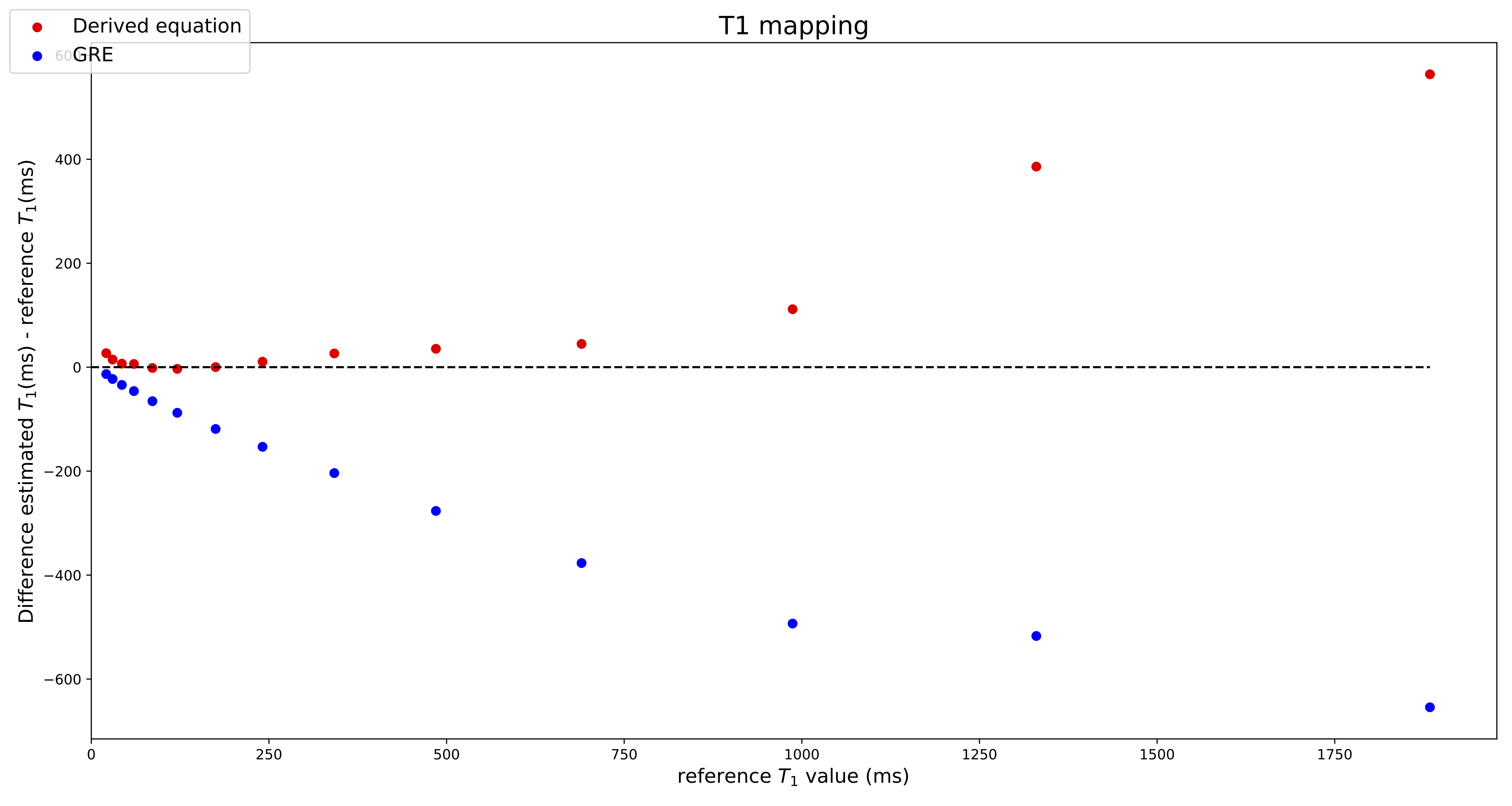
To validate the equation we scanned the NIST phantom (CaliberMRI, T1 reference values 10ms-1879ms) on a 3T system (Ingenia, Philips, Best, Netherlands) using a 16-channel head coil. Imaging was performed with a SGRE sequence with 24 RF pulses and four different flip angles (2°, 7°, 15°, 25°) (TR=10ms, TBlack-blood=13ms, TSpoil=6.3ms, TFat-saturation=82ms). K-space was fully sampled using the PROUD patch⁵ and each k-line was sampled 24 times before going to the next line. Separate images with data only from one RF pulse during each shot were then reconstructed using ReconFrame (Gyrotools GmbH, Switzerland). For the RF pulse for which the model differs most from SGRE (first pulse in the shot), T1 maps are acquired and a Bland-Altman plot is generated showing the difference between the estimated and ground truth T1 values for conventional SGRE fitting and our new approach. Additionally, the carotid artery of a healthy volunteer was imaged using the same acquisition technique to visually assess the strength of black-blood and fat suppression during the shot.

Results

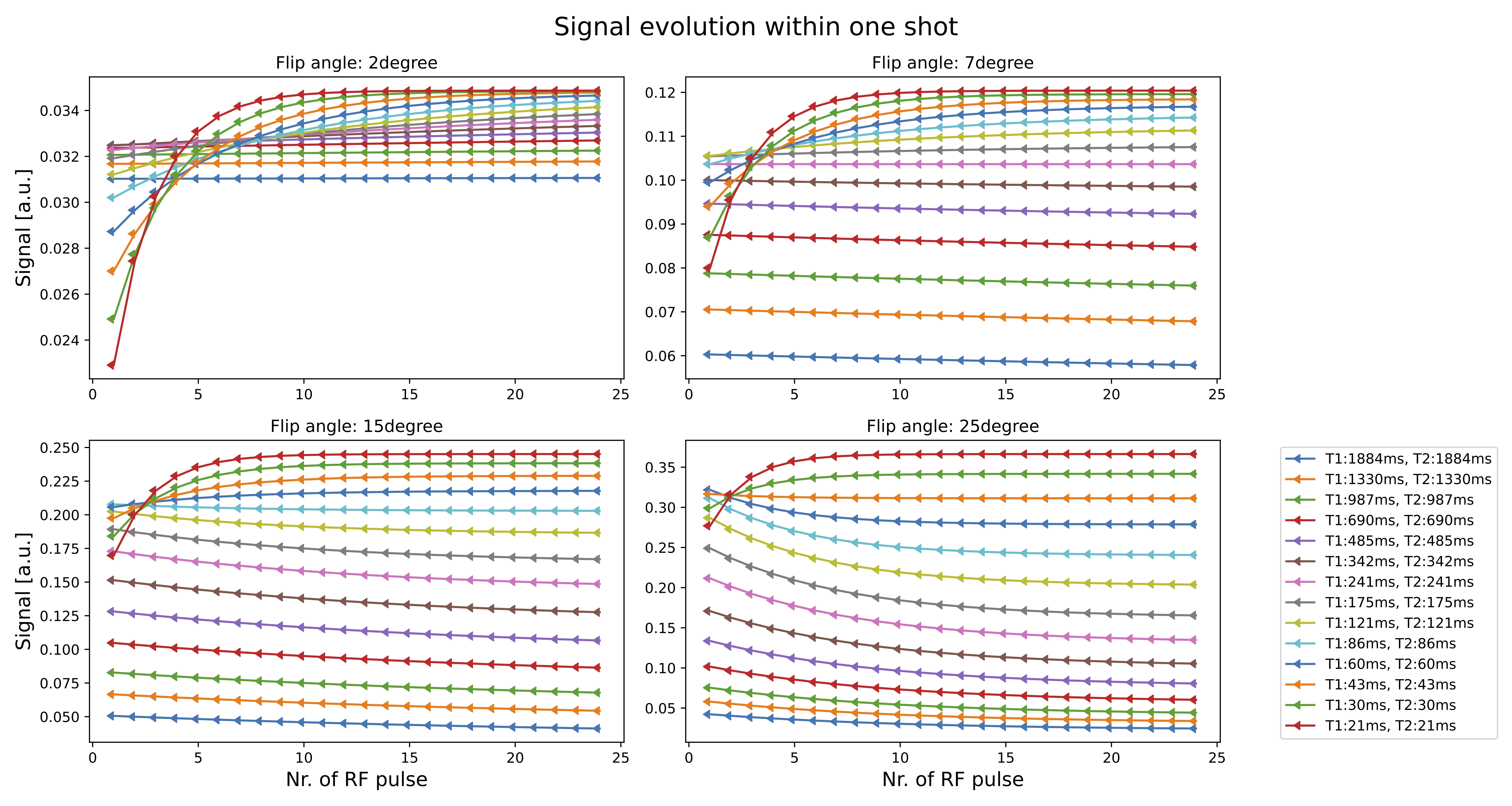
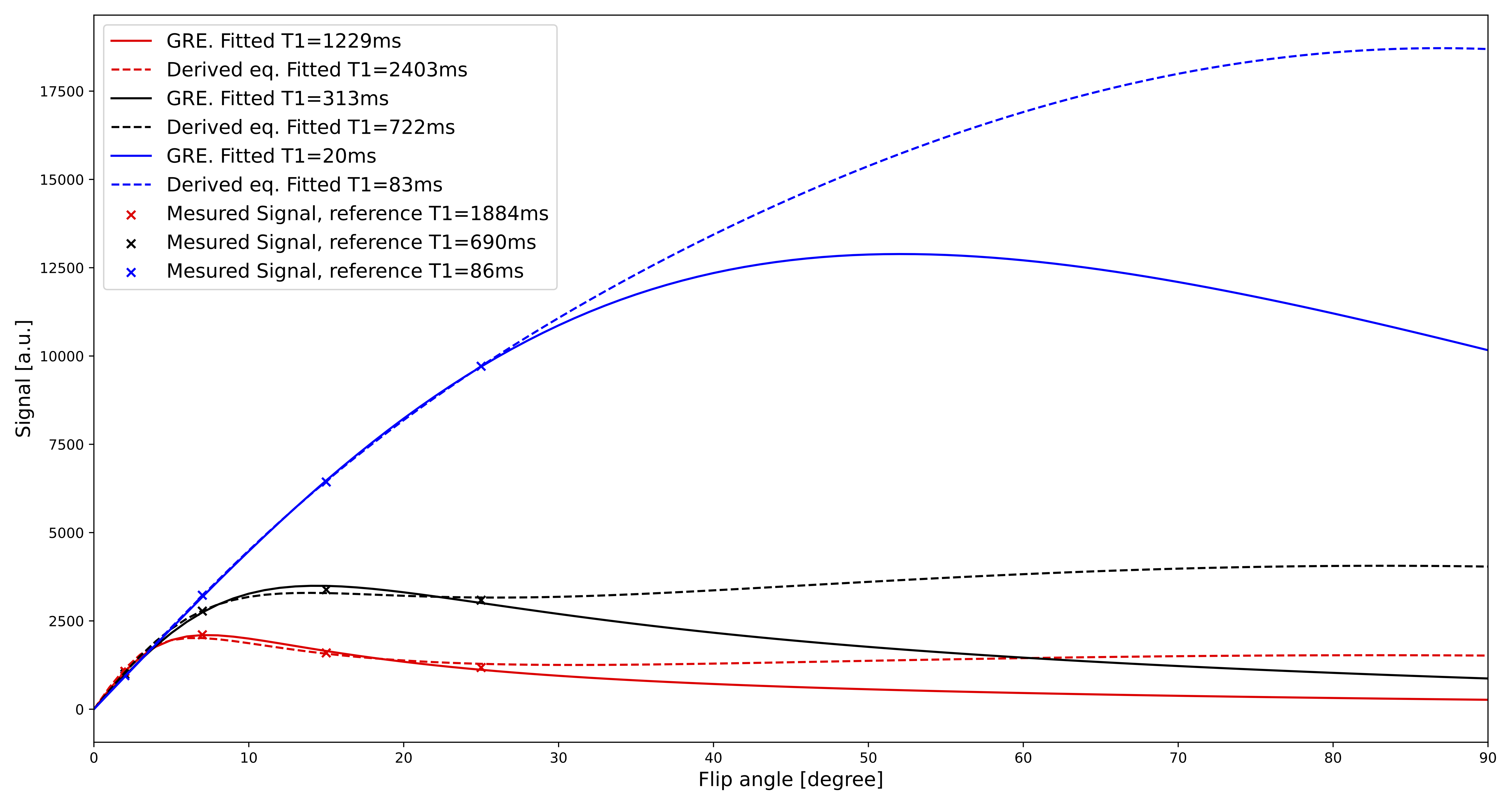
Spheres with shorter T1 and T2 values show a major signal change during the earlier RF pulses (Fig.2). For later RF pulses, the signal reaches a plateau which is similar to the signal from an SGRE. For the spheres with lower T1 values, the fit using the derived equation is closer to the reference values than using a normal SGRE signal equation (Fig.3). For higher T1 values, both fits deviate from the reference values. Although the measured data is described well by both models (Fig.4) for the flip angles measured, the T1 values estimated by SGRE deviate substantially.

Discussion

In this work, we derived an equation describing the signal evolution during an SGRE sequence with preparation pulses. The signal changes especially during the earlier RF pulses and differs from the values for later RF pulses, where it approaches signal from an SPGR sequence without prepulses. Depending on the acquisition settings, in particular for protocols that fill low k-lines first, it might be useful to take our new equation into account. One large disadvantage of our equation is the additional T2-dependence of the signal. Skipping early RF pulses during each shot returns the signal to (almost) SGRE and hence can overcome this dependency on T2, rendering T1 mapping less challenging. Important to consider then is the decreasing effect of preparation pulses as shown in the animation in Fig.5, where fat signal returns, while the blood suppression is visible throughout the entire shot.

Acknowledgements

No acknowledgement found.