3378

Identification of Subcortical White Matter Biomarkers in Multiple Sclerosis Patients using Machine Learning

Cristian Montalba^1,2,3, Raul Caulier-Cisterna^1,3, Pamela Franco^1,3, Tomás Labbé², Marcelo E Andia^1,2,3, Miguel Guevara⁴, Jean-François Mangin⁵, Juan Pablo Cruz², Ethel Ciampi^6,7, Claudia Cárcamo^7,8, Pamela Guevara⁴, Rodrigo Salas^3,9,10, and Sergio Uribe^1,2,3
¹Biomedical Imaging Center, Pontificia Universidad Catolica de Chile, Santiago, Chile, ²Radiology Department, School of Medicine, Pontificia Universidad Catolica de Chile, Santiago, Chile, ³Millennium Institute for Intelligent Healthcare Engineering - iHEALTH, Pontificia Universidad Catolica de Chile, Santiago, Chile, ⁴Faculty of Engineering, Universidad de Concepción, Concepción, Chile, ⁵UNATI, Neurospin, CEA, Université Paris-Saclay, Gif-sur-Yvette, France, ⁶Neurology Service, Hospital Dr. Sótero del Río, Santiago, Chile, ⁷Neurology Department, School of Medicine, Pontificia Universidad Catolica de Chile, Santiago, Chile, ⁸Interdisciplinary Center of Neurosciences, Pontificia Universidad Catolica de Chile, Santiago, Chile, ⁹Faculty of Engineering, Universidad de Valparaíso, Valparaíso, Chile, ¹⁰Biomedical Engineering School, Universidad de Valparaíso, Valparaíso, Chile

Synopsis

Keywords: Multiple Sclerosis, Machine Learning/Artificial Intelligence

Radiological biomarkers of cognitive impairment in Multiple Sclerosis (MS) are still scarce. This study aimed to identify subcortical white matter biomarkers of cognitive impairment related to verbal episodic memory in MS patients and healthy controls using a Machine Learning approach.

Introduction

Cognitive decline is recognized as a prevalent symptom of Multiple Sclerosis (MS), especially in episodic memory¹. These deficits are associated with grey matter atrophy and white matter lesions in subcortical areas^2-4. Clinical tests detect mild cognitive changes in specific cognitive domains. The Auditory Verbal Learning Test (AVLT) is a screening tool to detect changes in verbal episodic memory⁵. Current neurocognitive batteries may not identify early changes, precluding a timely diagnosis and treatment⁶.MR techniques improve the understanding of the development of cognitive impairment in relapsing-remitting MS (RRMS) patients⁷. Neuroimaging techniques, such as Diffusion Tensor Imaging (DTI), provide different indices to evaluate the axonal injury and demyelination, such as Fractional Anisotropy, Mean Axial, Axial Diffusivity, and Radial Diffusivity (FA, MD, AD, and RD, respectively)⁸. Therefore, a biomarker that could detect patients with cognitive deficits might benefit from early diagnosis and treatment.Machine Learning (ML) algorithms have shown promising results in classifying Magnetic Resonance Image (MRI) of patients with neurologic disorders^9,10. These approaches can be used to provide insights of relevant biomarkers with MRI, with the potential to be incorporated into routine clinical practice.In this study, we used an ML approach to identify subcortical white matter biomarkers between Healthy Controls with Cognitive Preserved (HC-CP) and RRMS patients with or without cognitive impairment (RRMS-CP, RRMS-CI, respectively), in verbal episodic memory as determined by the results from the AVLT test, with a classifier build using a ML approach.

Methods

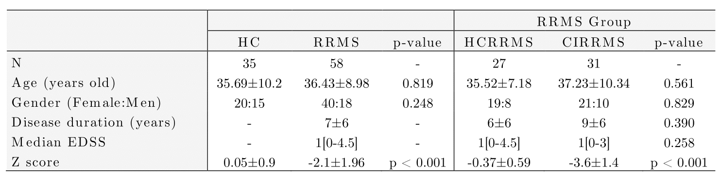
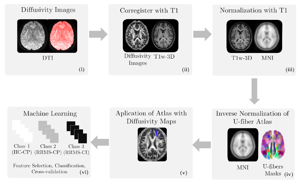
Diffusion-weighted and T1-weighted images were acquired in a 3T MRI scanner (Philips Ingenia, Best, Netherlands) in 35 HC (57% female) and 58 RRMS patients (69% female). The local ethics committee approved the study, and RRMS patients were diagnosed according to the 2017 McDonald's criterial⁷.Table 1 summarizes the demographic data. All patients were evaluated with an Expanded Disability Status Scale (EDSS) and verbal memory assessment using AVLTVIII⁵. All test scores were normalized in Z-scores. Using the Z-score, patients and healthy controls were categorized as HC-CP and RRMS-CP with a Z-score >= -1.5 and RRMS-CI with a Z-score < -1.5.Diffusion-weighted images were processed to obtain FA, AD, MD, and RD maps using DTI. T1-weighted images were used as an anatomical reference. All preprocessing steps were performed in SPM12¹². We used the LNAO-SWM79 U-fiber atlas as a mask to obtain the mean FA, AD, MD, and RD map to each subject's U-fiber¹³.Furthermore, classifiers were designed to select U-fiber maps that adequately separate HC-CP vs. RRMS-CP, RRMS-CP vs. RRMS-CI, and HC-CP vs. RRMS-CI and between the three classes. We used Sequential Forward Selection (SFS) as a feature selection algorithm to eliminate highly correlated or constant features that maximized accuracy¹⁴. The classifiers used were minimum distance, Linear Discriminant Analysis (LDA), k-Nearest Neighbors, Quadratic Discriminant Analysis, Mahalanobis distance, Support Vector Machine, Neural Network, and Random Forest (RF)¹⁵. The classification performance was evaluated using stratified 10-fold cross-validation, 90% training, and 10% testing. Confusion matrices were obtained from the results in each training and validation sample, calculating the accuracy of each strategy¹⁶. Also, we used t-Distributed Stochastic Neighbor Embedding (t-SNE) to visualize high-dimensional datasets (classification with features selected by SFS features)¹⁷. The strategy is summarized in Figure 1.

Results

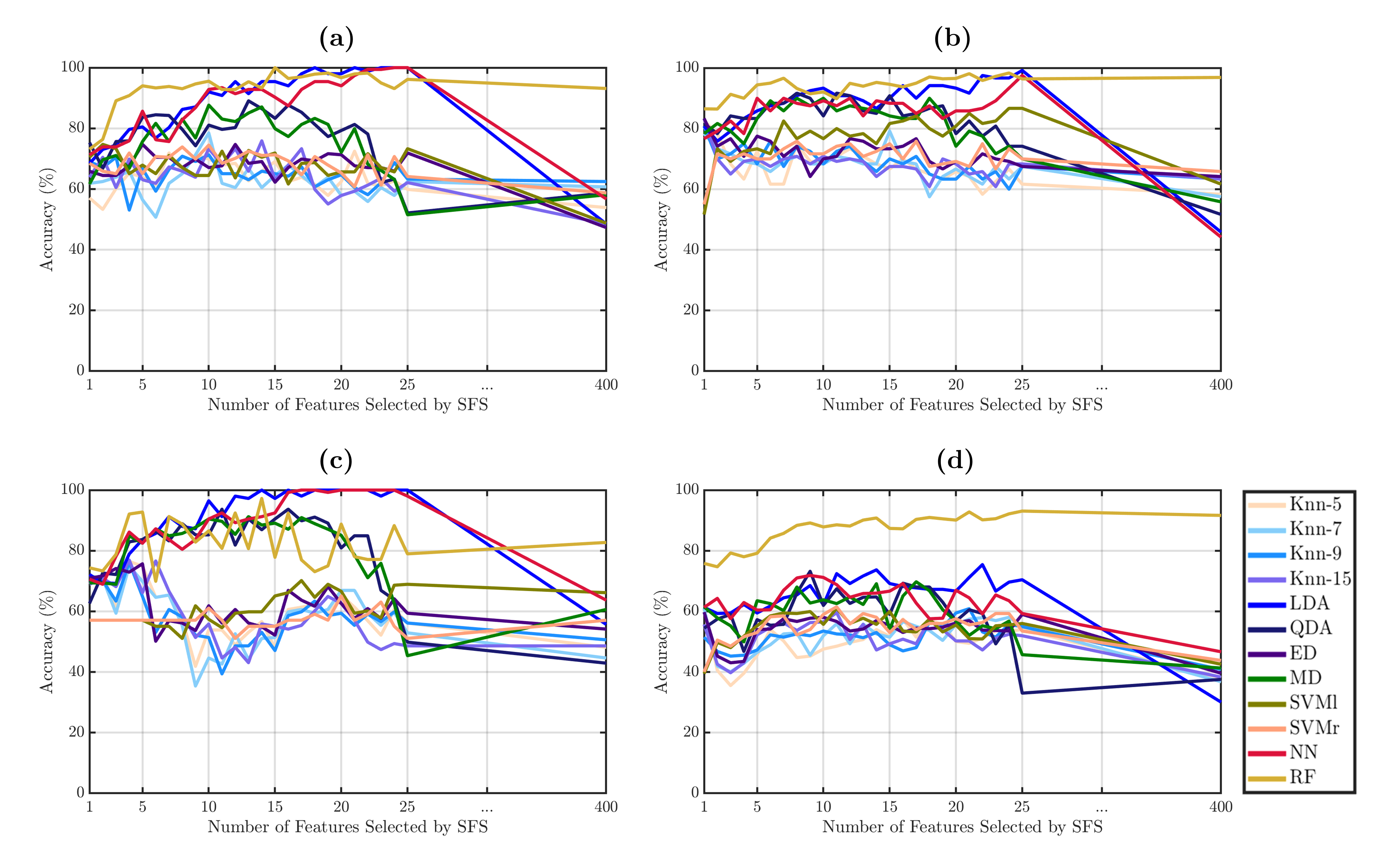
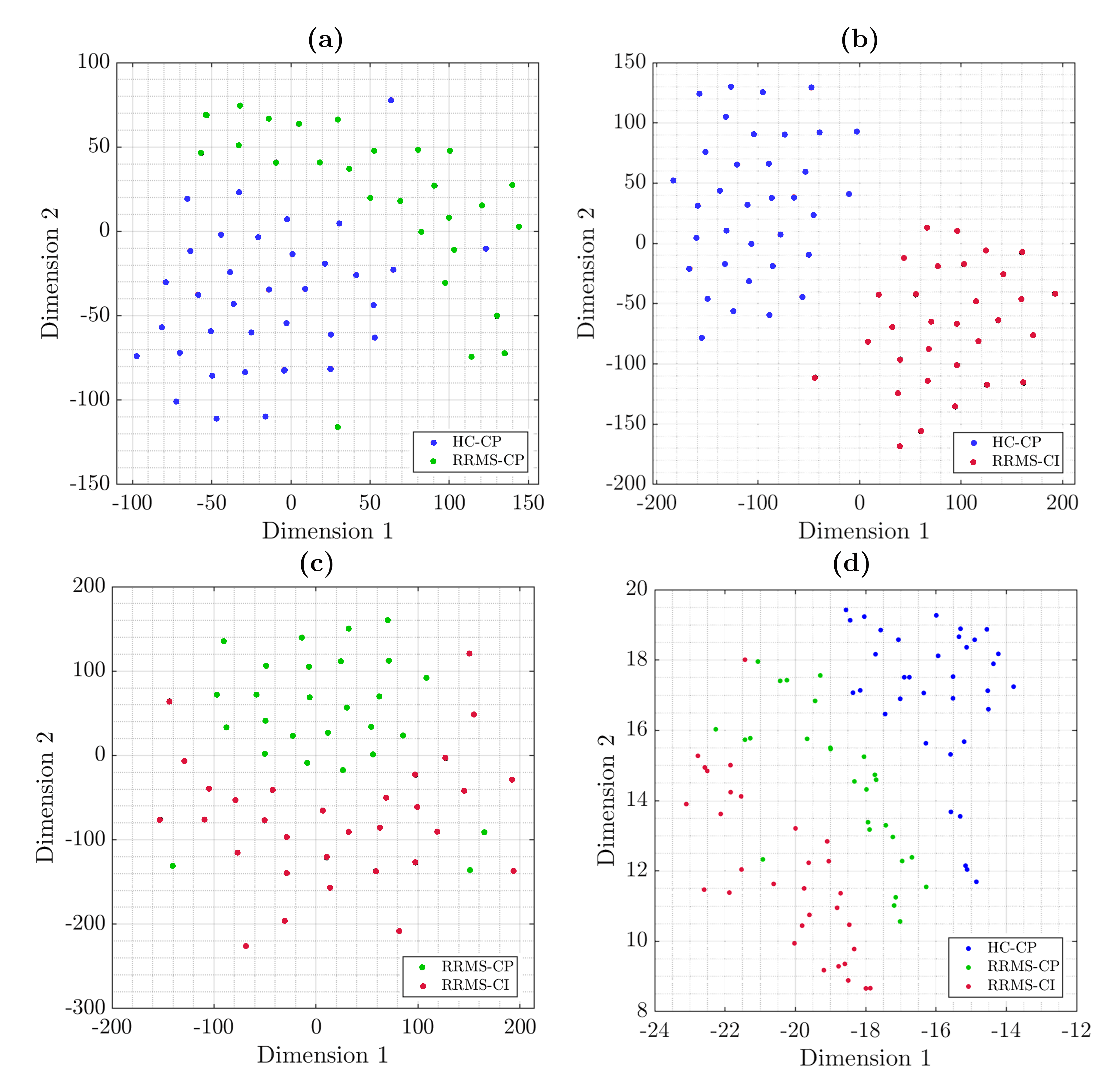
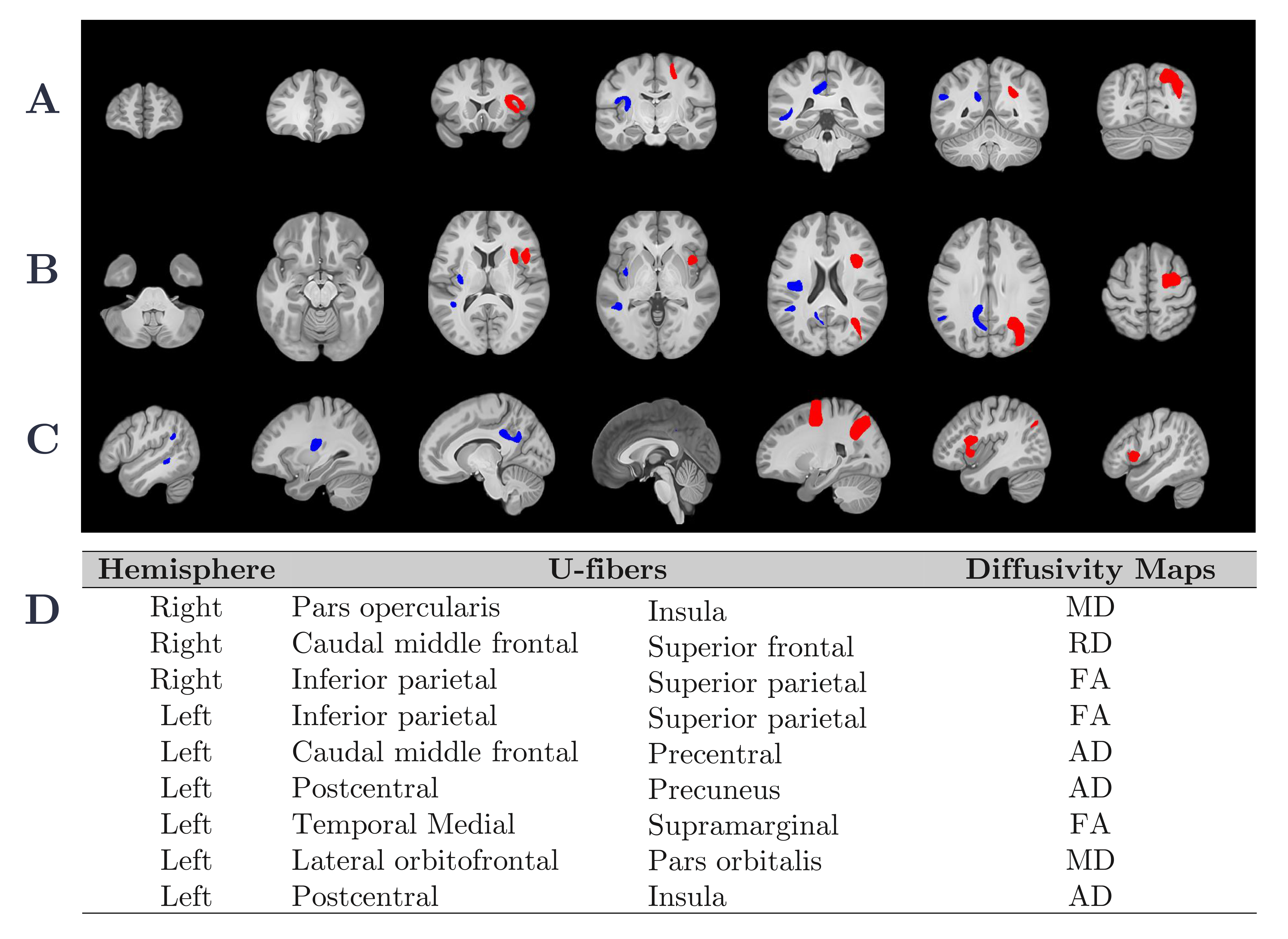
All strategies and classifiers are summarized in Figure 2. To evaluate the performance of the classifiers, we evaluated the accuracy percentage. Using features selected by SFS, RF reach the maximum accuracy with 15 features with accuracy of 100 ± 0% (Figure 3.a), LDA with 25 features with accuracy of 96.37 ± 1.5% (Figure 3.b), LDA with 14 features with accuracy of 97.23 ± 2.1% (Figure 3.c), and RF with 9 features with accuracy of 89.16 ± 2.5% (Figure 3.d), for HC-CP vs. RRMS-CP, HC-CP vs. RRMS-CI, RRMS-CP vs. RRMS-CI, and among three classes, respectively. The t-SNE results are shown in Figure 2. These results showed a good separation between the classes, that probes the results obtained from the previously analysis. Finally, Figure 4 shows the nine-top best nine-top performing features selected by SFS. These were MD: right pars opercularis insula and left lateral orbitofrontal pars orbitalis ; RD: right caudal middle frontal superior frontal, FA: right and left inferior parietal superior patient, and left temporal medial supramarginal, and AD: left caudal middle frontal precentral, postcentral precuneus and postcentral insula.

Conclusions

The ML strategy allows us to identify the most relevant subcortical areas that allow us to classify cognitive impairment from healthy controls based on verbal episodic memory. RF allowed us to identify automatically and robustly between HC and RRMS with and without cognitive impairment in verbal episodic memory, principally in frontal, parietal, and temporal areas. Miki Y, et al. studied the relation of the structural indemnity of subcortical brain areas related with the neuropsychological impairment, and found structural changes in the same brain areas³.The subcortical regions obtained with this ML approach allow us to identify patients with RRMS with early cognitive impairment caused by MS. This approach could be used to study other cognitive domains.

Acknowledgements

This work has been funded by projects PIA-ACT192064 and ICN2021_004 of the Millennium Science Initiative Program of the National Agency for Research and Development, ANID. The authors also thank the Fondecyt project 1181057 by ANID and PUENTE grant 2022-14 VRI, PUC. RC-C was funded by ANID Fondecyt Postdoctorado 2021 (Nº 3210305).

References

1. Benedict RHB, Amato MP, DeLuca J, et al. Cognitive impairment in multiple sclerosis: clinical management, MRI, and therapeutic avenues. Lancet Neurol. 2020 Oct;19(10):860-871. doi: 10.1016/S1474-4422(20)30277-5. Epub 2020 Sep 16. PMID: 32949546.

2. Brownell B, Hughes JT. The distribution of plaques in the cerebrum in multiple sclerosis. J Neurol Neurosurg Psychiatry. 1962;25:315–20.

3. Miki Y, Grossman RI, Udupa JK, et al. Isolated U- ber involvement in MS: preliminary observations. Neurology. 1998;50(5): 1301–6.

4. Lazeron RH, Langdon DW, Filippi M, et al. Neuropsychological impairment in multiple sclerosis patients: the role of (juxta) cortical lesion on FLAIR. Mult Scler. 2000;6(4): 280–5.

5. Bender HA, Cole JR, Aponte-Samalot M, Cruz-Laureano D, Myers L, Vazquez BR, Barr WB. Construct validity of the Neuropsychological Screening Battery for Hispanics (NeSBHIS) in a neurological sample. J Int Neuropsychol Soc. 2009 Mar;15(2):217-24. doi: 10.1017/S1355617709090250. Epub 2009 Feb 12. PMID: 19215638.

6. Sumowski JF, Benedict R, Enzinger C, et al. Cognition in multiple sclerosis: State of the eld and priorities for the future. Neurology. 2018 Feb 6;90(6):278-288. doi: 10.1212/WNL.0000000000004977. Epub 2018 Jan 17. PMID: 29343470; PMCID: PMC5818015.

7. Thompson AJ, Banwell BL, Barkhof F, et al. Diagnosis of multiple sclerosis: 2017 revisions of the McDonald criteria. Lancet Neurol. 2018 Feb;17(2):162- 173. doi: 10.1016/S1474-4422(17)30470-2. Epub 2017 Dec 21. PMID: 29275977.

8. Sbardella E, Tona F, Petsas N, et al. DTI Measurements in Multiple Sclerosis: Evaluation of Brain Damage and Clinical Implications. Mult Scler Int. 2013;2013:671730.

9. Klöppel S, Stonnington CM, Chu C, et al. Automatic classification of MR scans in Alzheimer’s disease. Brain 2008;131:681–689.

10. Wottschel V, Alexander DC, Kwok PP, et al. Predicting outcome in clinically isolated syndrome using machine learning. NeuroImage Clin 2015;7:281– 287.

11. Verikas A, Gelzinis A, Bacauskiene M: Mining data with random forests: a survey and results of new tests. Pattern Recognition 2011, 44(2):330–349.

12. Montalba C, Labbe, T, Andia M, et al. Evaluation of PASAT test performance and difusivity indices in U-fiber regions in healthy subjects and RRMS patients. 10. Proc. Intl. Soc. Mag. Reson. Med. 29 (2021).

13. Guevara M, Román C, Houenou J, et al. Reproducibility of superficial white matter tracts using di fusion-weighted imaging tractography. Neuroimage. 2017 Feb 15;147:703-725.

14.- Mery D. Computer Vision for X-Ray Testing: Imaging, Systems, Image Databases, and Algorithms, Springer (1st ed) 2015.

15.- Ciaburro G. MATLAB for Machine Learning: Practical examples of regression, clustering and neural networks, Publisher: Packt Publishing, 2017, ISBN: 978-1788398435

16.- Witten I and Frank E, Data mining: practical machine learning tools and techniques, San Mateo (2nd ed.), 2005.

17.- L. van der Maaten, G. Hinton, Visualizing Data using t-SNE, J. Mach. Learn. Res. 9 (86) (2008) 2579–2605.

Figures

Table 1. Demographical and clinical data of HC-CP, RRMS-CP, and RRMS-CI patients. Quantitative data are expressed as the mean ± SD. EDSS: Expanded disability status scale. P-values are for the analysis of the data. χ² for gender. T-test for the variance of age, disease duration, and Z-scores. Kruskall Wallis for EDSS.

Figure 1. Pre-processing steps realized to obtain the U-fiber diffusivity maps. (i) Segmentation of Diffusivity maps. (ii) Coregistration between diffusivity maps and T1w-3D image. (iii) Normalization of T1w-3D image to the MNI space. (iv) The deformation matrix of the normalized T1w-3D image was applied to the U-fiber masks in order to adapt to the diffusivity maps. (v) LNAO-SWM79 Atlas was adapted to each patient. (vi) Finally, a ML strategy was applied to recognize possible subcortical white matter biomarkers as a search problem of features and suitable classifiers.

Figure 2. Accuracy performance obtained from different classifiers in relation to the most relevant brain regions selected by SFS. Figura 2. KNN: k-Nearest Neighbors, LDA: Linear Discriminant Analysis, QDA: Quadratic Discriminant Analysis, ED: Eucludian Distance, MD: Mahannabolis Distance, SVMl: Suport Vector Machine lineal, SVMr: Support Vector Machine radial, NN: Neuronal Network, RF: Random Forest (a). HC-CP vs. RRMS-CP, (b). HC-CP vs. RRMS-CI, (c). RRMS-CP vs. RRMS-CI, and (d). Among three classes.

Figure 3. t-SNE: t-Distributed Stochastic Neighbor Embedding with the features selected by SFS that reach the maximum accuracy by the classifiers studies. (a). HC-CP vs. RRMS-CP, (b). HC-CP vs. RRMS-CI, (c). RRMS-CP vs. RRMS-CI, and (d). Among three classes. The red-color represent to RRMS-CI, the green-color represent to RRMS-CP and blue-color represent HC-CP.

Figure 4. The best accuracy results obtained from different combinations of U-fiber maps in all classes selected by SFS using RF, with an accuracy of 89.16 ± 2.5%. A. Coronal plane, B. Axial plane, C. Sagittal plane, D. Summary of the nine most relevant subcortical areas. Blue and Red colors represent the areas located in the left and right hemispheres, respectively.

Proc. Intl. Soc. Mag. Reson. Med. 31 (2023)

3378

DOI: https://doi.org/10.58530/2023/3378