Synopsis

Keywords: Machine Learning/Artificial Intelligence, Machine Learning/Artificial Intelligence, Model-Based Learning

The bSSFP sequence is intrinsically sensitive to T1 and T2, motion robust, and allows highly efficient data acquisition. Slow convergence in qMRI parameter fitting can potentially be mitigated by machine learning, which benefits greatly from the availability of accurate ground truth data. This work presents an unsupervised model-based NN that incorporates the analytical bSSFP signal equation into the training loop, thus avoiding the need for ground truth relaxometry measurements and enabling instantaneous multi-parametric submillimeter whole-brain mapping of T1 and T2. NN performance was compared to MIRACLE quantitatively for in silico noise corrupted data and qualitatively for in vivo data.

Introduction

Artificial neural networks (NNs) provide a fast alternative to traditional fitting approaches for multi-parametric quantitative magnetic resonance imaging (qMRI). However, long scan times and inefficient data acquisition schemes still limit the amount of available qMRI data for supervised NN learning, which requires ground truth data. The mixed sensitivity of the balanced steady-state free precession (bSSFP) sequence to both relaxometry metrics T1 and T2¹ makes it a promising tool for simultaneous relaxometry^2–4. Motivated by recent work using an analytical MRI model to simulate training data and to be integrated into the forward path of NN training⁵, we compare motion-insensitive rapid configuration relaxometry (MIRACLE²) to model-based training with simulated phase-cycled bSSFP (pc-bSSFP) data for simultaneous T1 and T2 mapping in silico and in vivo. Based on simulations, we further investigate the effects of different noise levels on the estimation performance of our NN and MIRACLE and qualitatively compare relaxometry estimates from high resolution pc-bSSFP in vivo data for both approaches.

Methods

In vivo data were acquired at 3T. 3D sagittal bSSFP data with 12 phase-cycles evenly distributed in the range (0, 2π): φj = π/12∙(2j-1), j = 1,2,…12 (isotropic resolution: 0.9x0.9x0.9 mm³, TR/TE = 5ms/2.5ms, total acquisition time: 16 min and 15 s) and TurboFLASH data with and without a preconditioning RF pulse (29s) for B1 were acquired.
Synthetic pc-bSSFP signals s were generated (Training/Validation/Testing, 200,000/40,000/16,000) using the forward bSSFP signal model s(p,u) in Equation 1 with parameters p = [T1, T2, B1⁺] (longitudinal relaxation time T1, transverse relaxation time T2 and scaling factor of transmit field B1⁺ = α_act / α_nom) and sequence parameters u = [TR, TE, α, Npc] (repetition time TR, echo time TE, flip angle α, number of phase cycle acquisitions Npc)⁶.

$$M_{ss}=M_0\frac{(1-E_1)(1-E_2e^{-i\phi})sin\alpha}{Ccos\phi+D}$$
With:
$$E_{1,2}=e^{-T{1,2}/TR}, C=E_2(E_1-1)(1+cos\alpha), D=(1-E_1cos\alpha)-(E_1-cos\alpha)E_2^2$$
and
$$\phi [0, 2\pi]=\pi / Npc * (2j -1)$$ with $$j=1,2,...Npc$$

Input parameter ranges for Equation 1 were sampled from a uniform distribution (T1: [1,2000] ms, T2: [1,500] ms, B1⁺: [0.7,1.3]) with an additional constraint of excluding T1 < T2 parameter combinations. Sequence parameters were fixed based on in vivo pc-bSSFP measurements (TR = 5 ms, TE = TR/2 ms, α = 15°, Npc = 12). Pc-bSSFP data were Fourier transformed to receive the Fn modes with various number of inputs for the NN (MIRACLE: [F_-1,F₀,F₁], NN: [F_-4,…,F₄], [F_-3,…,F₃], [F_-2,…,F₂], and [F_-1,F₀,F₁]). In silico and in vivo data matching was achieved by adjacent Euclidean distance normalization of the complex Fn modes along each voxel. Shown in Figure 1, both MIRACLE and NN take the absolute value of the Fn modes and an additional B1⁺ as input. In addition, synthetic datasets were corrupted with different noise levels σ (σ = A/SNR) based on an SNR range of [20,60,80,100,120,140,200] and A = 0.5 (approximated mean of [|F_-1|,|F₀|,|F₁|]). MIRACLE fitting was implemented using an iterative golden section search minimization⁷. Within the NN forward path, a multilayer perceptron of six hidden layers and rectified linear unit in each hidden layer was used to estimate the inverse signal model s^-(p,u) and infer the relaxometry parameters pnet = [T1, T2]. NN training was performed on synthetic data only, which took around 165min (300 epochs, batch size 32). In the forward path of a training loop, pnet together with the given input of B1⁺, was fed back into the signal model s(pnet,u) to derive the pc-bSSFP signal. The l2-norm was used to compare the Fn modes from the NN snet(pnet,u) with the original input from s(p,u). Data simulation, NN training and MIRACLE iterative fitting was implemented in Python 3.10.6. The quantitative mapping scheme is shown in Figure 1.

Results

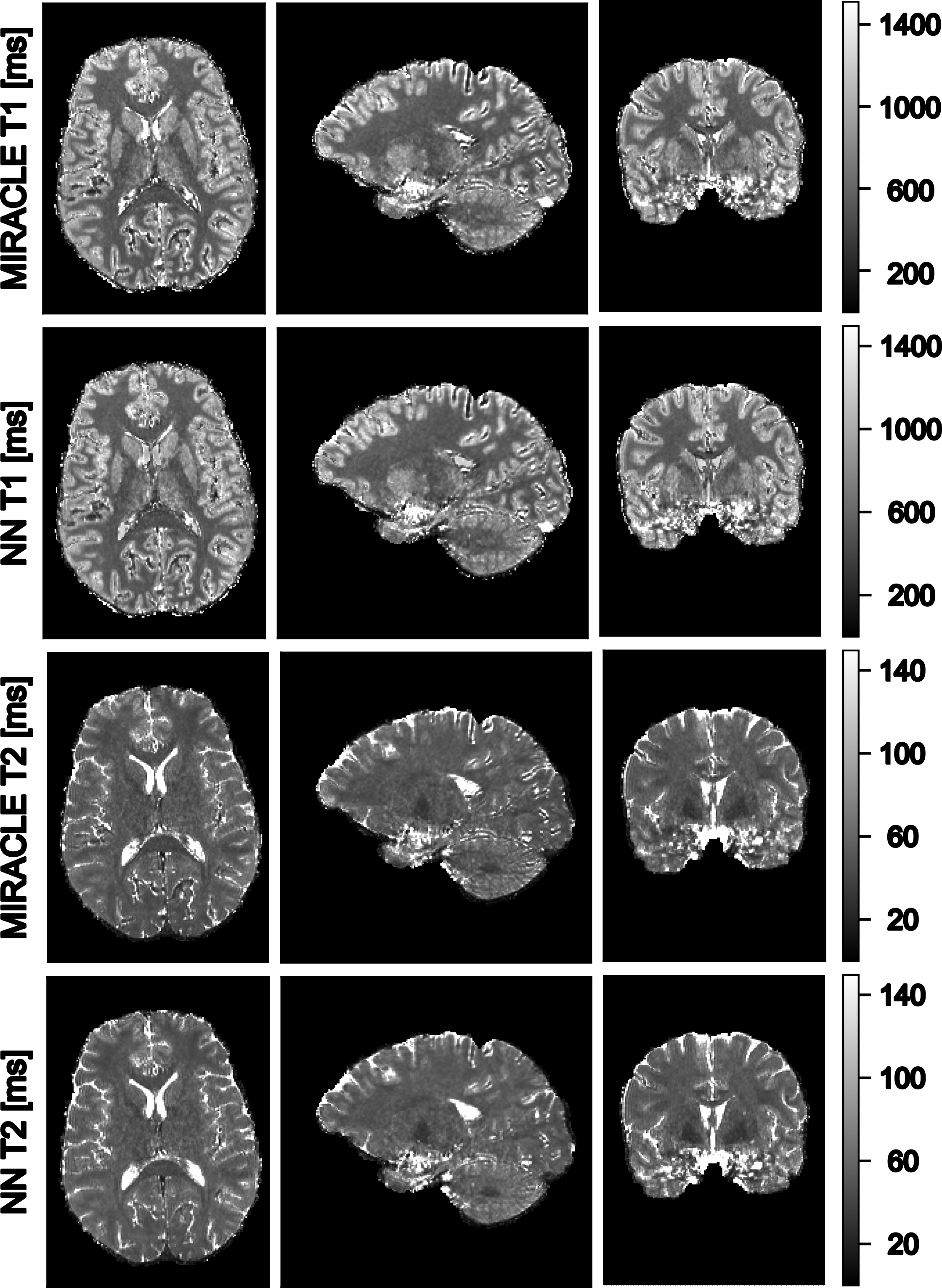
Shown in Figures 2 and 3, MIRACLE and NN estimations were validated on synthetic data using the coefficient of determination (CoD) and the root mean squared error (RMSE). If a noise-free signal is considered, MIRACLE outperforms each NN of different input sizes in T1 estimates but is inferior for T2. Adding noise to the signal, the NN is superior to MIRACLE and an increased number of Fn modes appears beneficial for NN input (Figure 2). Thus, the following results show estimations of NNs trained with an increased number of inputs (F_-4 to F₄, B1⁺). Figures 3 and 4 support the findings that MIRACLE estimation performance decreases with SNR while NNs trained at the respective SNR levels tend to be clearly more robust. Exemplary axial, sagittal, and coronal slices of in vivo whole brain T1 and T2 maps are shown in Figure 5 for MIRACLE and the NN. The estimation time for MIRACLE was ~75 seconds while that for the NN was ~1 second. Comparable qualitative results can be observed for both approaches.

Discussion and Conclusion

Model-based learning incorporates known analytical models into the learning process, eliminating the need for additional ground truth measurements. This reduces the large number of NN input and target data sets required for training based on measured in vivo data and potentially facilitates the clinical translation. With emphasis on the flexibility of adjusting sequence parameters and data distributions using in silico data paired with ultrafast inference times of multiple quantitative parameters, the proposed work proved that NNs are a valuable alternative to traditional model fitting approaches in multi-parametric qMRI.

Acknowledgements

No acknowledgement found.