3250
Repeatability of very low field MRI
Pavan Poojar1 and Sairam Geethanath1
1Accessible Magnetic Resonance Laboratory, Biomedical Imaging and Engineering Institute, Department of Diagnostic, Molecular and Interventional Radiology, Icahn School of Medicine at Mount Sinai, New York, NY, United States, New York, NY, United States
1Accessible Magnetic Resonance Laboratory, Biomedical Imaging and Engineering Institute, Department of Diagnostic, Molecular and Interventional Radiology, Icahn School of Medicine at Mount Sinai, New York, NY, United States, New York, NY, United States
Synopsis
Keywords: Data Acquisition, Low-Field MRI
Low-field MR scanners are low-cost, portable, and requires lesser space. In this study, we performed in vitro phantom repeatability study on a 48 mT scanner (Multiwave technologies) by scanning the phantom 3 sessions in a day (11 AM, 2 PM, and 5 PM) at 3 locations. During each scan, we measured the temperature, humidity, and F0 to see their effect on the image. We scanned 9 sequences in the study to monitor noise, F0 and B0. The difference in temperature and humidity was determined for each session.The line intensity profilesrevealed that VLF scanner produces consistent B0 maps and qualitative images.Purpose
To investigate the repeatability of very-low-field MRI using an invitro phantom to measure the transmit frequency, humidity, temperature and off-resonance and their effect on the resulting images.Methods
Study design: In-vitro phantom (Pro-MRI by Pro Lab) was scanned in a VLF scanner (50mT, Multiwave Technologies SA, France) for 3 times a day over a period of 10 days (except weekends). Each day 3 scans were performed in three different sessions: session 1 starts at 11 AM, session 2 at 2 PM and session 3 at 5 PM. Before and after each session temperature (oc) and humidity (%RH) were measured at 3 locations: location 1: centre of the bore (front of phantom), location 2: front of the bore, location 3: centre of the room (room temperature and humidity). These measurements were carried out inorder to see the effect of temperature and humidity. The scanner and the phantom was not moved throughout the repeatability study. The scanner was turned on in the morning before the session 1 and turned off after the session 3. This was repeated for all the 10 days. Acquisition: The VLF repeatability protocol includes 9 sequence: 1) Monitor noise: this is to measure the noise and it was less than 0.07 μdB. 2) findf0: this is find the central frequency. This was performed before and after each scan. 3) 3D turbo spin echo (TSE, (1)) with echo shift of 1 μs and 50us (2) 4) 3D TSE with echo shift of 50 μs. Both 4 and 5 sequences were used to reconstruct the B0 map. The acquisition parameters were: TR/TE - 500/20 ms, echo train length - 4, field of view (fov) - 230x230x125 mm3, resolution - 1.5x1.5x5 mm3, number of averages - 1, bandwidth (BW) - 50 kHz with acquisition time of ~8 minutes for each 3D TSE scan. 6) 3D TSE to compare the T1 weighted qualitative images over 3 sessions and 10 days. The acquisition parameter and acquisition time was same as that of sequence 5 except the BW - 40 kHz. Sequence 7 and 8 were same as sequence 4 and 5. With these sequences, B0 map was generated before and after the TSE sequence. The total scan time for the entire session was ~40 minutes. Reconstruction and analysis: The B0 maps were generated by calculating the phase difference with the help of 3D TSE with and without echo shift of 49us. The generated maps were further masked to remove the background. The 3D qualitative T1 weighted volume was reconstructed using 3D FFT. All reconstructions were performed in Python. The delta temperature and humidity were calculated for each session and plotted. For f0, the delta f0 was calculated for each sequence (total of 5 values), converted to Hz from mHz and computed the mean of the delta f0 for all the three sessions. Similarly, the mean B0 values were calculated and plotted across all sessions.Results
Figure 1 (a-c) shows the plot of delta temperature over all 10 days, 3 sessions and for all 3 locations. Similarly, figure 1 (d-f) shows the plot for delta humidity (%RH) for all 3 locations. Figure 1 (g) shows the mean delta f0 for all the 3 sessions. Figure 2 (a-b) shows the B0 maps obtained before and after 3D TSE scan. Each column represents the days and row represents individual session. It can be visually observed that most of the maps are in similar range except for the day 6 of session 1 (before and after). These 4 B0 maps were not in range as shown in with blue hollow box. Hare, the background value was updated to -5000 Hz to for better visualization of the map. Figure 3 (a-b) show the quantification of B0 maps by calculating the mean of the B0 map values for before and after 3D TSE sequence. It can be observed from the the plots that both for 6th day and 10 day for the session 1, the mean B0 values were out of range (both in before and after 3D TSE). This is in line with the figure blue boxes in the figure 2. Figure 4 shows the qualitative images of the phantom obtained from 3D TSE sequence. Each row shows represents session and each column represents day. The last column shows the line intensity profile of the phantom for the row pixels shown with orange line in first image. It can be observed from the line intensity profile that all images produces similar profile with some noise. It can be seen that all image images possess geometrical distortion (shown with yellow arrow on first image).Discussion and conclusion
From figure 2 and 4, it is clear that the VLF scanner produces consistent B0 maps and qualitative images. The qualitative images shown here were not corrected with the distortion. The limitations of this study include, B0 correction, understanding the effect of humidity on the images, quantifying contrast and signal to noise ratio (SNR). Current and future work is addres all the above mentioned limitations.Acknowledgements
Multiwave Technologies SAReferences
1. O’Reilly, T., Teeuwisse, W.M., de Gans, D., Koolstra, K. and Webb, A.G., 2021. In vivo 3D brain and extremity MRI at 50 mT using a permanent magnet Halbach array. Magnetic resonance in medicine, 85(1), pp.495-505.Koolstra,
2. K., O’Reilly, T., Börnert, P. and Webb, A., 2021. Image distortion correction for MRI in low field permanent magnet systems with strong B0 inhomogeneity and gradient field nonlinearities. Magnetic Resonance Materials in Physics, Biology and Medicine, 34(4), pp.631-642.
Figures
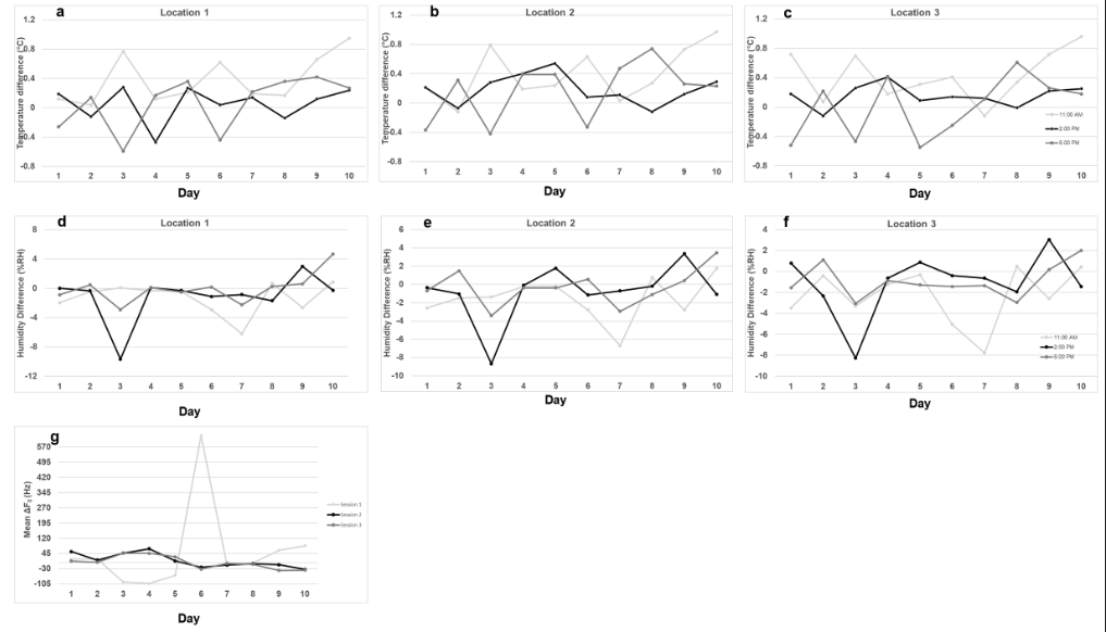
Figure 1: Difference in temperature, humidity and F0 for all 3 sessions over 10 days.
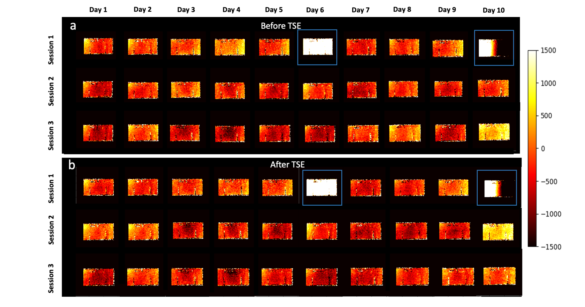
Figure 2: B0 maps (a) before 3D TSE (b) after 3D TSE sequence over 10 days and across 3 sessions.
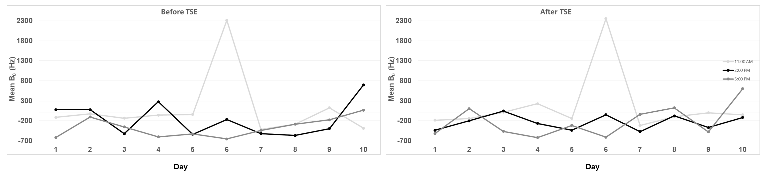
Figure 3: Mean B0 changes before and after 3D TSE sequence for 10 days across 3 sessions.
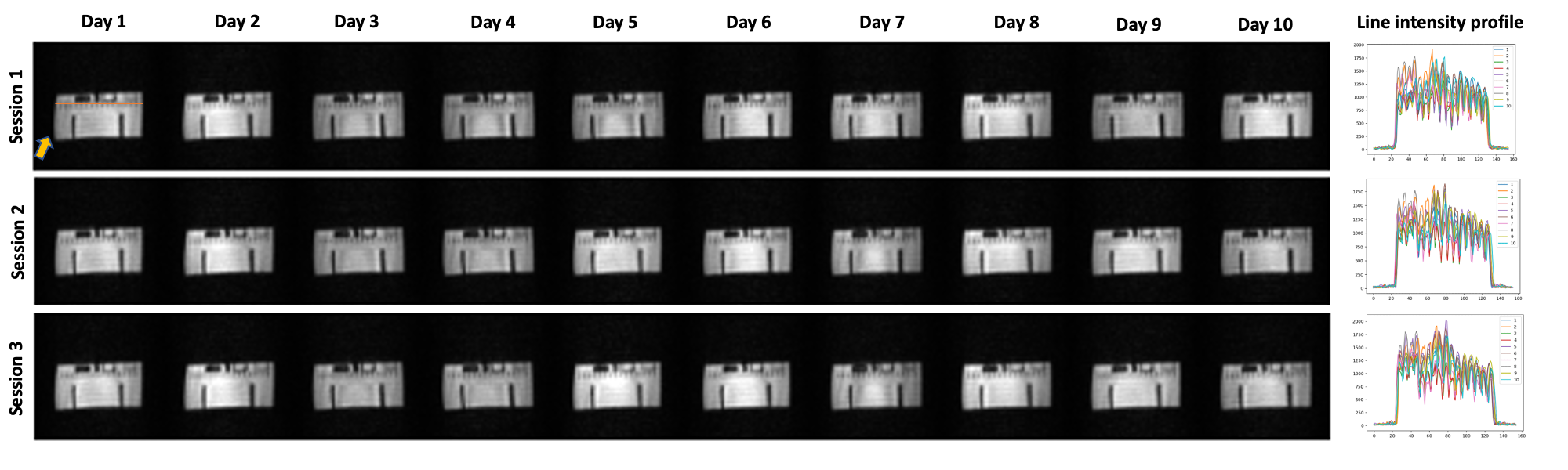
Figure 4: 3D TSE qualitative images for all three sessions over 10 days. The line intensity plot is shown in the last column. The yellow arrow shows the distorted region of the image.
DOI: https://doi.org/10.58530/2023/3250