Synopsis

Keywords: Data Analysis, Magnets (B0), optimization; static field inhomogeneity; artifact correction

Many methods deployed for Magnetic Resonance Imaging (MRI) suffer from degraded image quality when the static magnetic field ($$$B_0$$$) is nonuniform, as $$$B_0$$$ inhomogeneity causes different types of image artifacts and distortions. Image correction methods require a prior estimate of the field map. In this work, we study the problem of static $$$B_0$$$ inhomogeneity estimation from distorted and undistorted image pairs, despite undistorted images being noisy. The estimated field map is later utilized to correct distorted images. The efficacy of the proposed approach is demonstrated for different encoding methods in the presence of large magnetic field inhomogeneity via extensive simulations.

Introduction

To correct different artifacts generated due to the inhomogeneity of $$$B_0$$$, several approaches have been proposed, for which the field map information is necessary^1,2. Recently, convolutional neural networks (CNNs) have been utilized to acquire prior information about phase errors in the training data and unnecessitate accurate field map information^3,4. When the off-resonance frequency induced by the magnet increases, the blurring disperses information more broadly with respect to the number of voxels, which significantly degrades CNN-based approaches. Instead of CNN-based methods, we propose an analytical approach to better understand the problem of large magnet inhomogeneity estimation using a training set of distorted and undistorted image pairs taken to be at the same physical location within the magnet. To estimate the field map induced by the magnet, a linear transformation of the field map is estimated first. Next, a golden-section search and regularization via the expansion of spherical harmonics are proposed to extract off-resonance frequencies. The estimated $$$B_0$$$ inhomogeneity is leveraged to propose an image correction scheme.

Problem Formulation and Methods

The inhomogeneity-sensitive encoding matrix with phase errors is denoted by $$$\mathbf{A}_f^s\in\mathbb{C}^{m\times n}$$$, where $$$[\mathbf{A}_f^s]_{ij}=e^{-\iota 2\pi f_j(T_E+t_i) }e^{-\iota 2\pi \mathbf{k}_i\cdot\mathbf{r}_j }$$$. One obtains the signal equation for the $$$c^{\text{th}}$$$ coil in matrix form as follows:
$$\hspace{-9.5cm}\mathbf{y}_c^k=\mathbf{A}_f^s\mathbf{S}_c\mathbf{x}^k+\boldsymbol{\epsilon}_{c}^k, $$where $$$\mathbf{S}_c\in\mathbb{C}^{n\times n}$$$, $$$\mathbf{x}^k\in\mathbb{C}^{n\times 1}$$$, and $$$\boldsymbol{\epsilon}_{c}^k\in\mathbb{C}^{m\times 1}$$$ are the diagonal coil sensitivity, $$$k^\text{th}$$$ ground-truth image, and the additive noise. A distorted image is generated under the assumption that there is no $$$B_0$$$ inhomogeneity:$$\hspace{-9.5cm}\tilde{\mathbf{x}}^k= \arg\min_{\tilde{\mathbf{x}}^k} \quad \sum_{c=1}^{C}\frac{1}{2}\lVert \mathbf{A}_0^s\mathbf{S}_c\tilde{\mathbf{x}}^k-\mathbf{y}_c^k\rVert_2^2+\frac{1}{2}\lVert \mathbf{R}\tilde{\mathbf{x}}^k\rVert _2^2, $$where $$$\mathbf{A}_0^s $$$ and $$$\mathbf{R}$$$ are the standard encoding matrix and a regularization matrix to improve the condition number⁵, respectively. Moreover, we consider a dataset of (possibly noisy) fully sampled measurements acquired using an encoding method resistant to magnetic field inhomogeneity (e.g., 3D phase encoding or single point imaging^6,7,8). One obtains the vector of undistorted measurements as $$$\mathbf{w}_c^k=\mathbf{A}_0^p\mathbf{S}_c\mathbf{x}^k+\boldsymbol{\zeta}_{c}^k$$$. We formulate the following optimization problem to jointly estimate images in $$$\mathbf{X}=\{\mathbf{x}^k \}_{k=1}^K, K\geq n$$$, and the field map $$$\mathbf{A}_f^s$$$:$$\min_{\mathbf{X},\mathbf{A}_f^s} \hspace{1cm}\sum_{k=1}^{K}\sum_{c=1}^{C}\frac{1}{2}\lVert\mathbf{A}_0^p\mathbf{S}_c\mathbf{x}^k-\mathbf{w}_c^k\rVert_2^2\hspace{12cm}(1a)\\ \hspace{.3cm}\textrm{s.t.} \hspace{1.3cm}\tilde{\mathbf{x}}^k=\arg\min_{\tilde{\mathbf{x}}^k} \sum_{c=1}^{C}\frac{1}{2}\lVert\mathbf{A}_0^s\mathbf{S}_c\tilde{\mathbf{x}}^k-\mathbf{y}_c^k\rVert_2^2+\frac{1}{2}\lVert \mathbf{R}\tilde{\mathbf{x}}^k\rVert_2^2,\hspace{7.6cm}(1b)$$where $$$\mathbf{A}_f^s$$$ is embedded in $$$\mathbf{y}_c^k$$$. Using the first order optimality condition and setting the gradient to zero, we can simplify (1b) to the following minimization:$$\min_{\mathbf{X},\boldsymbol{\Psi}}\hspace{0.5cm} \lVert (\mathbf{\Gamma}+\mathbf{R}^H\mathbf{R})\tilde{\mathbf{x}}^k-(\mathbf{V}\circ \mathbf{\Psi})\mathbf{x}^k\rVert_2^2, \hspace{12cm}(2)$$where $$$\mathbf{\Gamma}=\mathbf{V}\circ ((\mathbf{A}_0^s)^H\mathbf{A}_0^s) $$$, $$$\mathbf{\Psi }= (\mathbf{A}_0^s)^H\mathbf{A}_f^s $$$, $$$\mathbf{V}=\sum_{c=1}^{C}(\mathbf{s}_c)^*(\mathbf{s}_c)^T$$$, $$$\circ$$$ denotes Hadamard product, and $$$\mathbf{s}_c$$$ is the vector of diagonal of $$$\mathbf{S}_c$$$. To approximate the solution, $$$\mathbf{x}^k $$$ is obtained from (1a) via gradient methods⁵, and using that, $$$\boldsymbol{\Psi }$$$ is estimated from (2). For one element of $$$\boldsymbol{\Psi }$$$, we have $$$[\mathbf{\Psi}]_{oj}=\sum_{i=1}^{m}e^{-\iota 2\pi f_j(T_E+t_i)}e^{\iota 2\pi \mathbf{k}_i\cdot(\mathbf{r}_o-\mathbf{r}_j)}$$$. Accordingly, we use the following equivalent minimizations to estimate off-resonance frequencies: $$\min_{\{f_j\}_{j=1}^n} \hspace{0.5cm} \sum_{j=1}^{n}\sum_{o=1}^{n}\Big|[\hat{\mathbf{\Psi}}]_{oj}-\sum_{i=1}^{m}e^{-\iota 2\pi f_j(T_E+t_i)}e^{\iota 2\pi \mathbf{k}_i\cdot(\mathbf{r}_o-\mathbf{r}_j)}\Big|^2\equiv\min_{\{g_j\}_{j=1}^n} \hspace{0.5cm } \sum_{j=1}^{n} \sum_{o=1}^{n}\Big|[\hat{\boldsymbol{\Psi}}]_{oj}-\sum_{i=1}^{m}e^{-\iota g_j(i +\frac{T_E}{\Delta t})}e^{\iota 2\pi \mathbf{k}_i\cdot(\mathbf{r}_o-\mathbf{r}_j)}\Big|^2, $$where $$$ g_j =2\pi f_j\Delta t$$$. The advantage of the equivalent problem is that $$$-\pi\leq g_j\leq\pi$$$, which shrinks the variable domain. We obtain the neighborhood in which the cost function is unimodal around the global minimizer using a grid search in $$$[-\pi,\pi]$$$. Next, we implement a golden-section search method⁹ to extract the global minimizer. We obtain $$$ \hat{f}_j= \frac{\hat{g}_j }{2\pi\Delta t}$$$. After we estimate off-resonance frequencies, we regularize them by projecting them to the subspace spanned by the 2D spherical harmonics up to the third order¹⁰. With the estimated inhomogeneity, we approximate $$$\boldsymbol{\Psi}$$$. To unblur/correct an image, fixing $$$\boldsymbol{\Psi}$$$, we solve (2) with respect to $$$\mathbf{x}^k $$$. If $$$(\mathbf{V}\circ\mathbf{\Psi})$$$ is rank deficient, we use $$$\ell_0$$$ or $$$\ell_1$$$ regularization to obtain efficient solutions⁵.

Simulation Results

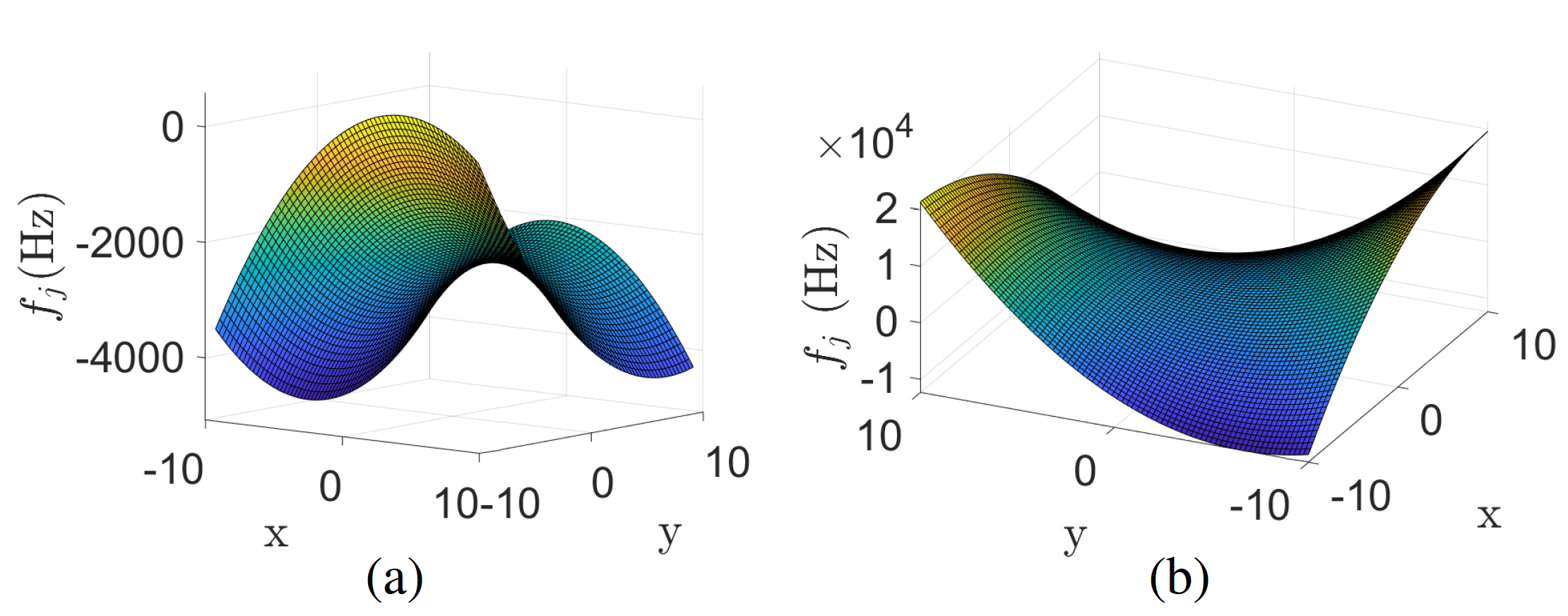
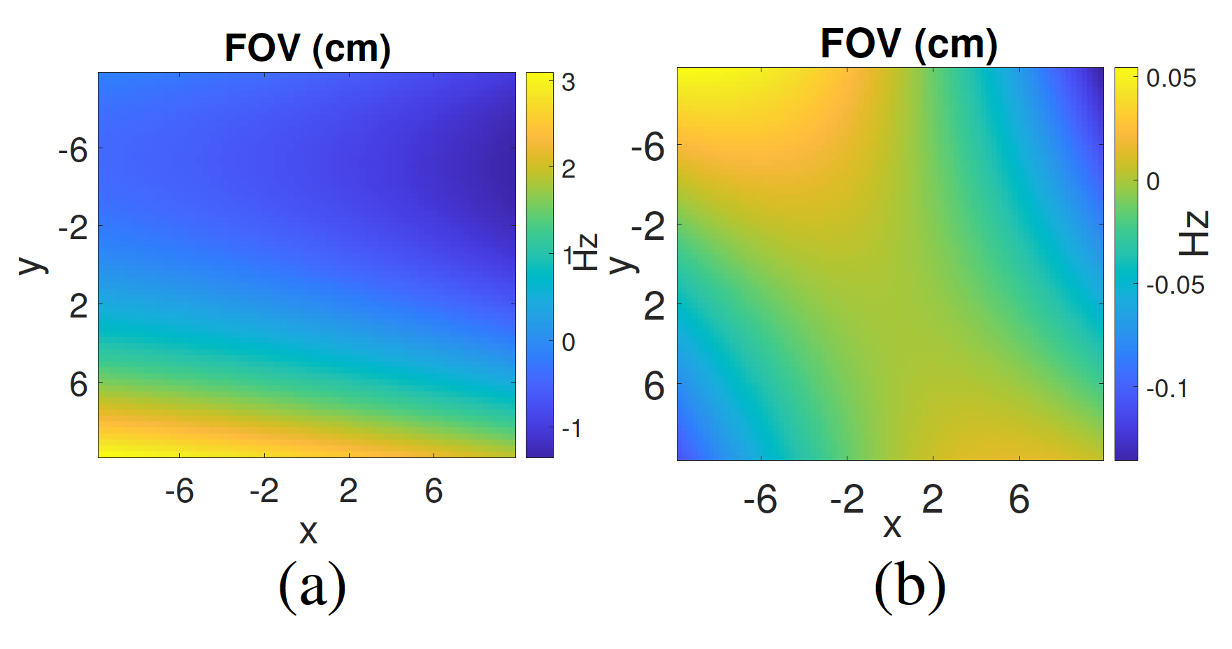
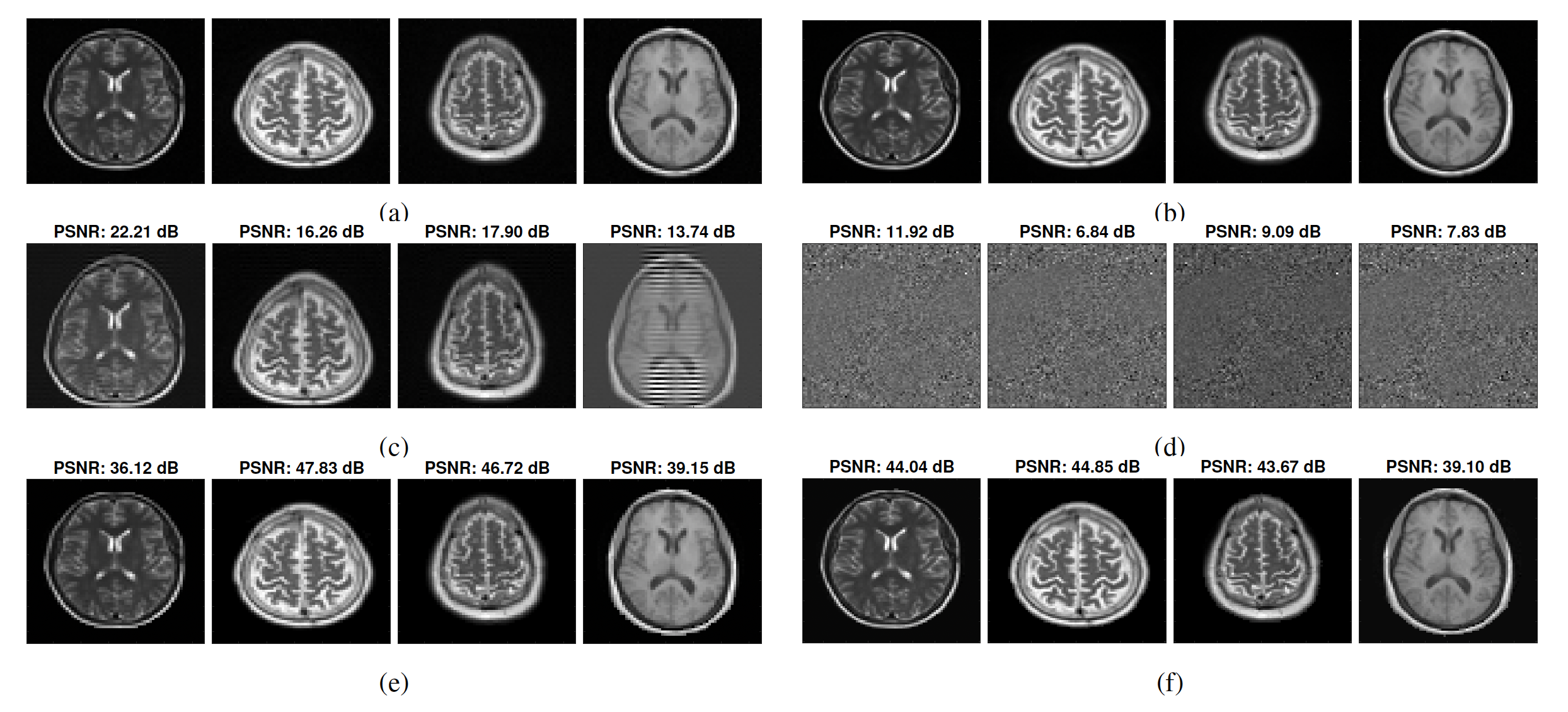
We evaluate the performance of the proposed method for multi-shot Cartesian and single interleaf-spiral encodings. To obtain a $$$B_0$$$ map, large $$$B_0$$$ inhomogeneity was experimentally generated by deliberately mis-setting room temperature shims. A 3D Cartesian k-space was sampled using 2D phase-encoding and 1D frequency encoding using an MP-SSFP sequence¹¹ to refocus inhomogeneity with low peak RF amplitude. The resulting $$$B_0$$$ inhomogeneity was mapped by taking two measurements: once with the center of the frequency encoded readout aligned to the center of the spin echo, and once with the center of the readout gradient shifted $$$100$$$ $$$\mu s$$$ from the center of the spin echo. For analysis, axial slices of the 3D images were used, with in-plane FOV of $$$19.2\:\text{cm}\times 19.2\:\text{cm}$$$, $$$64\times 64$$$ k-space points, readout dwell time $$$= 33.6$$$ $$$\mu s$$$, with one coil. For the spiral trajectory, k-space samples are generated via MIRT¹² and undersampled $$$4x$$$. We set the dwell time $$$= 4\:\:\mu s$$$ and $$$FOV=20\:\text{cm}\times 20\:\text{cm}$$$. Eight coils are utilized. Surfaces of off-resonance frequencies are depicted in Fig. 1 for both encodings. Accordingly, we add phase errors to the standard encoding matrices and use them to generate $$$10,000$$$ distorted images⁴ from images in NYU DICOM¹³. The error of the off-resonance frequency estimation in each voxel is depicted in Fig. 2. Separately for both encodings, we use (2) and depict corrected test images, which are from multiple slices with different contrasts, in Fig. 3.

Concluding Remarks

This paper studied field map estimation using two datasets of a common set of objects. We proposed a novel method to estimate the off-resonance frequency in each voxel. Estimated 2D off-resonance frequencies are regularized through spherical harmonics that represent the surface of off-resonance frequencies. The estimated field map is used to design an image deblurring scheme.

Acknowledgements

This work was supported in part by the National Institutes of Health Grant U01 EB025153 and Grant P41 EB027061.

References

[1]. J. A. Fessler, S. Lee, V. T. Olafsson, H. R. Shi, and D. C. Noll, “Toeplitzbased iterative image reconstruction for MRI with correction for magnetic field inhomogeneity,” IEEE Trans. Signal Process., vol. 53, no. 9, pp.3393–3402, Sep. 2005.

[2]. B. P. Sutton, D. C. Noll, and J. A. Fessler, “Fast, iterative image reconstruction for MRI in the presence of field inhomogeneities,” IEEE Trans. Med. Imag., vol. 22, no. 2, pp. 178–188, Feb. 2003.

[3]. D. Y. Zeng, J. Shaikh, S. Holmes, R. L. Brunsing, J. M. Pauly, D. G. Nishimura, S. S. Vasanawala, and J. Y. Cheng, “Deep residual network for off-resonance artifact correction with application to pediatric body MRAwith 3D cones,” Magn. Reson. Med., vol. 82, no. 4, pp. 1398–1411, 2019.

[4]. Y. Lim, Y. Bliesener, S. Narayanan, and K. S. Nayak, “Deblurring for spiral real-time MRI using convolutional neural networks,” Magn. Reson. Med., vol. 84, no. 6, pp. 3438–3452, 2020.

[5]. J. A. Fessler, “Optimization methods for magnetic resonance image reconstruction: Key models and optimization algorithms,” IEEE Signal Process. Mag., vol. 37, no. 1, pp. 33–40, Jan. 2020.

[6] M. Halse, J. Rioux, S. Romanzetti, J. Kaffanke, B. MacMillan, I. Mastikhin, N. J. Shah, E. Aubanel, and B. J. Balcom, “Centric scan SPRITE magnetic resonance imaging: optimization of SNR, resolution, and relaxation timemapping,” Magn. Reson. Med., vol. 169, no. 1, pp. 102–117, 2004.

[7] S. Emid and J. H. N. Creyghton, “High resolution NMR imaging in solids,” Physica B+C, vol. 128, no. 1, pp. 81–83, 1985.

[8] M. Halse, D. J. Goodyear, B. MacMillan, P. Szomolanyi, D. Matheson, and B. J. Balcom, “Centric scan SPRITE magnetic resonance imaging,” Magn. Reson. Med., vol. 165, no. 2, pp. 219–229, 2003.
[9]. C. F. Gerald and P. O. Wheatley, Applied numerical analysis, Pearson/Addison-Wesley, 2004.
[10]. R. Gruetter and C. Boesch, “Fast, noniterative shimming of spatiallylocalized signals in vivo analysis of the magnetic field along axes,” J. Magn. Reson., vol. 96, no. 2, pp. 323–334, Feb. 1992.

[11]. S. Patz, S. T. S. Wong, and M. S. Roos, “Missing pulse steady-state free precession,” Magn. Reson. Med., vol. 10, no. 2, pp. 194–209, 1989.

[12]. J. A. Fessler, “Michigan image reconstruction toolbox,” Available [Online]: https://web.eecs.umich.edu/~fessler/code/mri.htm.
[13]. J. Zbontar, F. Knoll, A. Sriram, and T. Murrell, et al., “fastMRI: An open dataset and benchmarks for accelerated MRI,” arXiv preprintarXiv:1811.08839, 2018.