Synopsis

Keywords: CEST & MT, CEST & MT

Sensitivity encoding (SENSE) is often adopted to accelerate image acquisition for various MRI sequences, including APTw. This is further accelerated with SENSE with compressed sensing (called CS-SENSE), but the image quality degrades to some extent. We collected both SENSE- and CS-SENSE-APTw images and trained a generative model with residual learning to generate SENSE images from CS-SENSE images. The generated results were proved to be highly similar to SENSE-APTw images and less noisy than both SENSE- and CS-SENSE-APTw images. With a larger dataset, we can train more robust models and eventually replace SENSE- with CS-SENSE for a speedup of ~50%.

Introduction

Amide proton transfer-weighted (APTw) imaging, a type of chemical exchange saturation transfer (CEST) MRI,^1-4 is a protein-based molecular imaging technique.⁵ This technique has been successfully applied to brain tumors and many other diseases.^6-11 Currently, clinical APTw imaging has relatively longer acquisition time and is highly sensitive to motion. Sensitivity encoding (SENSE)¹² has been widely adopted in APTw imaging to speed up the acquisition, while still preserving satisfactory image quality. Recently, compressed sensing (CS) was further introduced to achieve even faster acquisition (called CS-SENSE), but the image quality degraded with a higher acceleration factor (AF). Previous studies have demonstrated that a CS-SENSE AF of 4 is acceptable for APTw MRI.^{13, 14} In this work, using SENSE-APTw images with an AF of 2 as the ground truth, we trained a neural network, which takes CS-SENSE-APTw images with an AF of 4 as the input, to generate images towards the ground truth. If the generated images have desirable quality, we may replace SENSE- with CS-SENSE and save nearly half of the acquisition time.

Method

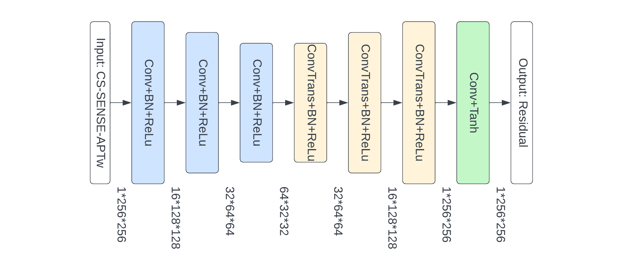
MR imaging was performed on a Philips 3T MRI scanner. A recommended 3D APTw imaging sequence¹¹ (saturation power = 2 μT; saturation time = 2 sec; TR = 6.5 sec; FOV = 212×192 mm²; 15 slices; slice thickness = 4 mm; matrix = 120×118, reconstructed to 256×256; SENSE = 2 or CS-SENSE = 4) was used to acquire APTw images. 63 patients with gliomas (male 41, female 22; age 53.5±13.9 years, ranged from 26-80 years) were included in our study and they were randomly divided into the training (50 patients) and testing (13 patients) sets. For each patient, SENSE- and CS-SENSE-APTw images were co-registered and skull-stripped, and the voxel values were normalized to [0, 1]. Each APTw image has 15 slices which were used as 15 separate 2D images.

CS-SENSE uses undersampling of k-space data to accelerate acquisition and the result is different from that acquired by SENSE, as there is an information loss in the undersampling process. Notably, to restore SENSE images using CS-SENSE images, we did not generate SENSE-APTw images themselves, as it was found harder to train with. Instead, we trained a convolutional autoencoder to learn the difference mapping between paired SENSE and CS-SENSE data (i.e., SENSE minus CS-SENSE). Subsequently, in the inference stage, the generated residuals from the autoencoder were added to the input CS-SENSE-APTw images to get the estimation of SENSE-APTw images. The architecture of the convolutional autoencoder was shown in Figure 1. It used 3 convolutional and transposed convolutional layers for under-sampling and up-sampling, which can extract features at both high and low levels while preserving more texture details than models using pooling layers.

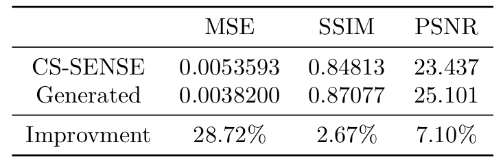
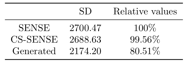
We employed mean squared error (MSE), structural similarity index measure (SSIM), and peak signal-to-noise ratio (PSNR) as the metrics to evaluate an image's similarity to corresponding ground truth (SENSE-APTw image). Lower MSE and higher SSIM and PSNR indicate higher similarity. The standard deviation (SD) of image signal intensities was used to estimate the level of noise. Lower SD indicates lower level of image noise.

Results and Discussion

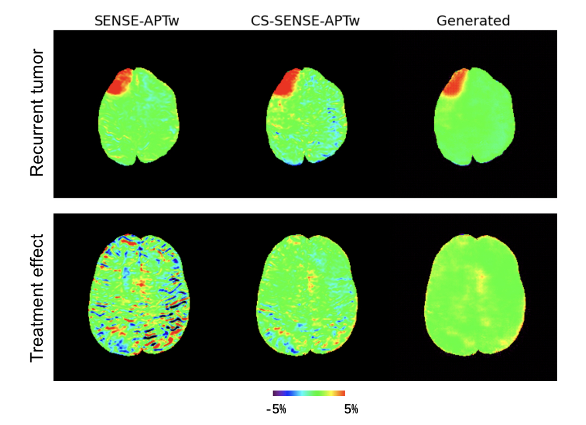
Two representative examples of the acquired SENSE-APTw and CS-SENSE-APTw images, as well as generated APTw images were illustrated in Figure 2. The first case (with recurrent anaplastic oligodendroglioma) proved the model’s capability to generate a high-quality APTw image using the undersampled one, with a visible noise level reduction; the second case (with treatment effect) demonstrated the model’s robustness to the motion artifact. The average metric values in the testing set were depicted in Table 1. Quantitatively, our model can not only accurately generate the high-quality SENSE-APTw images from CS-SENSE-APTw images, but can also reduce the noise level by approximately 19% compared to SENSE- and CS-SENSE APTw images (Table 2).

The size of the dataset is now small and it should further be verified whether the model can generate desirable results for any possible input. However, the preliminary results show that this work is a good start to our ultimate goal of completely replacing SENSE with CS-SENSE for faster APTw acquisition.

Conclusion

A convolutional autoencoder model with residual learning has been built to generate APTw images from CS-SENSE-APTw images using SENSE-APTw images as the ground truth. The generated images were proved to be highly similar to the ground truth and less noisy than both the input and the ground truth on average.

Acknowledgements

The authors thank our clinical collaborators for help with the patient recruitment and MRI technicians for assistance with MRI scanning. This study was supported in part by grants from the NIH.