3118
Digital Reference Objects with BART1Institute of Biomedical Imaging, Graz University of Technology, Graz, Austria, 2German Centre for Cardiovascular Research (DZHK), Partner site Göttingen, Göttingen, Germany, 3Department of Interventional and Diagnostic Radiology, University Medical Center Göttingen, Göttingen, Germany
Synopsis
Keywords: Software Tools, Software Tools
Digital Reference Objects (DRO) are important for developing imaging and reconstruction techniques especially in medical imaging applications. They allow a stepwise increase in complexity during testing of methods by simulating reproducible datasets.
In this work we present a variety of tools the BART toolbox provides for the creation and simulation of DROs. We present a workflow for designing DROs with Bézier curves using vector graphics applications which are then imported into BART.
Furthermore, we show simulation of analytical k-space data with 2D and 3D coil sensitivities and combining them with simulated signal curves to obtain k-space data for complex scenarios.
Introduction
In this work, we describe the creation of advanced Digital Reference Objects (DRO) with the BART toolbox [1].Building on work about DROs based on Bézier curves and their analytical Fourier representation by Guerquin-Kern et al. [2], we developed a framework to design DRO geometries with scalable vector graphic (SVG) applications such as Inkscape [3], extract the information of the Bézier curves and import it to BART's DRO geometry interface. These geometries can then be used to compute analytical k-space signals for complex shapes, also taking realistic coil sensitivities into account. Individual geometric components of a DRO can be combined with simulated signal evolutions to create temporal signal representations of measured objects.
Based on this framework, we created a new brain DRO with four different components.
To improve support for testing advanced parallel imaging, we also extended BART's built-in 2D coil sensitivities by adding a model for 3D sensitivities for a 64-channel head coil.
Geometry Design and Import
Realistic geometries for DRO require a generic description.Here we focus on the work by Guerquin-Kern et al. [2] describing MRI signals not just in image space $$$c_j(x)\rho(x)$$$ but also in k-space $$$\mathcal{F}(c_j\rho)(\omega)$$$ for multiple receive coils $$$j=1,...,N$$$ and density $$$\rho$$$.
In order to model MR data on arbitrary trajectories and avoid inverse crimes, we exploit the polynomial representation of the Bézier curve and sample it in image and k-space by using the Fourier convolution theorem
$$
\mathcal{F}(c_j\rho)(\omega)=\mathcal{F}(c_j)*\mathcal{F}(\rho)(\omega)\tag{1}.
$$
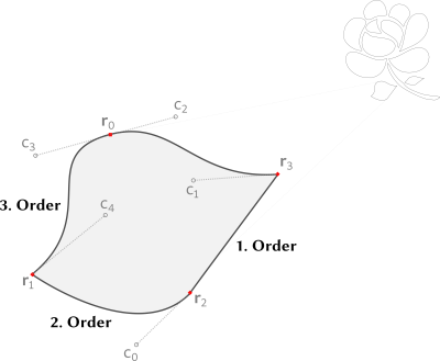
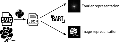
Complex geometries can be designed with any scalable vector graphics application, such as the open-source Inkscape program [3]. We developed an automated pipeline converting geometries to arrays of Bézier curve control points of order up to 3 of the form
$$
\rho(x)=\sum_{m=1}^M\rho_m(x)
$$
with non-overlapping domains $$$\text{dom}(\rho_l)\cap\text{dom}(\rho_m)=\emptyset\forall l\neq m$$$ (compare Figure 1). These arrays are stored in JSON format and can then be imported by BART.
The whole pipeline is shown in Figure 2.
Coil Sensitivities
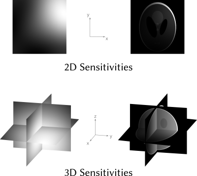
Coil sensitivity maps $$$c_j$$$ are smooth and their Fourier representation reduces, therefore, to a few coefficients simplifying the computation of equation $$$(1)$$$. For both cases, 2D and 3D, the values $$$\mathcal{F}(c_j)(\omega),j=1,...,64$$$ were precomputed and are accessible in BART for simulation of multi-channel signals (Figure 3).The precomputed profiles were obtained from a fully sampled 3D Cartesian FLASH acquisition with a 64 channel head coil on a Siemens Skyra 3T system. The precomputation was done in BART by solving the non-linear inverse problem [4]
$$
\min_{x}||Ax-y||^2_2+\alpha_1S(c_1,...,c_{64})+\alpha_2||\rho||_2^2,
$$
where $$$x=(\rho,c_1,...,c_{64})$$$, the operator $$$A$$$ represents the parallel MRI forward model, the measured data is $$$y$$$ and the Sobolev norm $$$S$$$ enforces smoothness of the $$$c_j$$$.
Temporal Signal Representations of DROs
For simulations of MRI measurements the temporal evolution of the magnetization has to be computed and combined with the geometry and coil profiles. In BART, geometry and signal creation are split in individual tools as shown in Figure 4.While the geometry interface can break objects like the brain phantom shown in Figure 4 into their individual components $$$1\leq m\leq M$$$, the simulation interface provides tools for analytical signal $$$s_m(x,t)$$$, Extended Phase Graph, Runge-Kutta Solver and State-Transition Matrix simulation [5,6,7].
We compute the signal of each geometric component and then obtain the final DRO with
$$
\sum_{m=1}^M s_m(x,t) \rho_m(x).
$$
This can be done in image or frequency space, can include coil sensitivity simulation $$$c_j\cdot \rho_m\cdot s_m$$$ and supports non-Cartesian sampling trajectories. The separation of geometry $$$\rho_m$$$ and signal function $$$s_m$$$ increases the flexibility of the interface.
Overall, BART provides the following tools for creating simulations:
- signal: Simulation of analytical signals
- epg: Extended Phase Graph Simulation
- sim: Solution of the Bloch Equations using a Runge-Kutta Solver and State-Transition Matrix Simulation
- noise: Simulation of noise
- traj: Creation of various Cartesian and non-Cartesian trajectories
- phantom: Creation of complex geometries with 2D and 3D coil profile simulation with up to 64 channels
Conclusion
This work presents a range of functionality which the BART toolbox provides for creating and simulating DROs in image and frequency domain, simulation of coils, noise and MR signals.A framework for designing geometries and importing them into BART is presented, simplifying the creation of complex geometries. Three dimensional coil sensitivities were added, extending the simulation to 3D with up to 64 channels. As an example, we show the creation of a human brain DRO with complex geometry.
Acknowledgements
Nick Scholand and Martin Schilling contributed equally to this abstract.
This work was partially funded by NIH under grant U24EB029240.
We acknowledge funding by the "Niedersächsisches Vorab" funding line of the Volkswagen Foundation and the Sonderforschungsbereich (SFB) 1456 with project 432680300.
References
[1] M. Uecker et al. Software Toolbox and Programming Library for Compressed Sensing and Parallel Imaging. ISMRM Workshop on Data Sampling and Image Reconstruction, Sedona 2013.
[2] M. Guerquin-Kern et al. Realistic Analytical Phantoms for Parallel Magnetic Resonance Imaging. IEEE Trans. Med. Imaging. 2012;31(3):626-636
[3] Inkscape Project. (2020). Inkscape. Retrieved from https://inkscape.org
[4] M. Uecker et al. Image reconstruction by regularized nonlinear inversion--joint estimation of coil sensitivities and image content. Magn. Reson. Med. 2008 Sep;60(3):674-82.
[5] C. Look and D.R. Locker. Time saving in measurement of NMR and EPR relaxation times. Rev. Sci. Instrum. 1970;41(2):250-251.
[6] J. Hennig et al. Calculation of flip angles for echo trains with predefined amplitudes with the extended phase graph (EPG)‐algorithm: principles and applications to hyperecho and TRAPS sequences. Magn. Reson.Med. 2004;51(1), 68-80.
[7] N. Scholand et al. Quantitative Magnetic Resonance Imaging by Nonlinear Inversion of the Bloch Equations. arXiv:2209.08027
Figures


Figure 4: MRI simulations in BART.
Geometric and signal components, $$$\rho_m(x)$$$ and $$$s_m(x,t)$$$, are created separately. The individual simulation of $$$\rho_m(x)\cdot s_m(x,t)$$$ results in the DRO $$$\sum_m\rho_m(x)s_m(x,t)$$$. The resulting simulation is presented as representative frames of the temporal evolution of the signal for a digital brain DRO for a single receive coil. The frames show ringing artifacts because the simulation makes use of an analytical expression to compute a correct Fourier representation of the geometric shapes.