3110
High efficient DTI reconstruction network with flexible diffusion directions
Zejun Wu1, Jiechao Wang1, Zunquan Chen1, Zhigang Wu2, Jianfeng Bao3, Shuhui Cai1, and Congbo Cai1
1Department of Electronic Science, Xiamen University, Xiamen, China, 2Philips Healthcare, Shenzhen, China, 3the First Affiliated Hospital of Zhengzhou University, Zhengzhou, China
1Department of Electronic Science, Xiamen University, Xiamen, China, 2Philips Healthcare, Shenzhen, China, 3the First Affiliated Hospital of Zhengzhou University, Zhengzhou, China
Synopsis
Keywords: Image Reconstruction, Diffusion Tensor Imaging
Deep learning has been used in diffusion tensor imaging (DTI) to fast reconstruct diffusion parameters. However, diffusion-weighted images (DWIs) as network input must maintain diffusion gradient direction consistency during training and testing for deep-learning-based DTI parameter mapping. A dynamic-convolution-based network was developed to achieve generalized DTI parameter mapping for flexible diffusion gradient directions. This proposed method uses dynamic convolution kernels to embed diffusion gradient direction information into feature maps of the corresponding diffusion signal. The results indicate that the proposed method can reconstruct high-quality DTI-derived maps from six diffusion gradient directions.Introduction
Diffusion tensor imaging (DTI) can be used to non-invasively investigate the orientation and structural connectivity of nerve fiber bundles, living white matter, and white matter bundles. Recently, deep neural networks have been widely applied for DTI reconstruction, and some deep-learning-based methods (e.g., DeepDTI1, and SuperDTI2), which use only six-direction diffusion-weighted images (DWIs), have been proposed to reduce scan time. However, these networks require that the diffusion gradient directions of the reconstruction data should be the same as the training data, which significantly limits their application. In the DiffNet method3, diffusion signals are normalized in a q-space and then projected and quantized, producing a matrix as an input for the network to achieve generalization. Nevertheless, DiffNet is a voxel-wise fitting and cannot use adjacent voxels for noise robustness. In addition, part of the information is lost because of overlapping in projection. In this work, different from existing approaches that fix kernels after training, we implemented a dynamic-convolution-based network to get the dynamical kernel parameters conditioned by the DWIs and diffusion direction information. Compared to DiffNet method, the results of the proposed method have a lower normalized root mean squared error (NRMSE) and a higher peak signal-to-noise ratio (PSNR) in DTI parameter maps for 6 diffusion gradient directions.Methods
Data acquisition: The data were obtained from the Human Connectome Project (HCP).4 There were 203 subjects in total, 136 for training, 46 for validation, and 21 for testing. T1-weighted images and DWIs with two b values (b = 0, 1000 ms/μm²) and 90 diffusion gradient directions were used for this study. Every subject had 145 slices, and the size of each slice was 174 x 145.Network: The input (Figure 1) of the network were: a T1-weighted image for preventing blurring and offering more structural information5, one b = 0 image, and six b = 1000 ms/μm² DWIs along 6 diffusion directions were randomly selected from the first 60 directions in HCP (6 of the last 30 directions in HCP for testing). We implemented a dynamic-convolution-based model to achieve generalized reconstruction for various diffusion gradient directions. The DWIs ($$$ W $$$) were aggregated into a one-dimensional vector via global average pooling (GAP). Moreover, the vector was concatenated with the diffusion direction vector ($$$ V $$$). By specifying the parameters of dynamic convolution layers ($$$ θ $$$), the concatenated vector was convolved and fully connected ($$$ φ $$$) to get the kernel parameter. This process is expressed as follows:$$ \omega = φ(GAP(W)||V; \theta_φ) $$ where $$$ θ_φ $$$ represents the weights and the biases of the dynamic convolution layers. The kernel parameters ω were allocated to three dynamic convolution layers. And the DWIs become feature maps (FM) through the three layers. This method mapped the six parameters ($$$ D_{xx} $$$, $$$ D_{yy} $$$, $$$ D_{zz} $$$, $$$ D_{xy} $$$, $$$ D_{xz} $$$, $$$ D_{yz} $$$) of diffusion tensor.
Evaluation: The average of 18 b = 0 images and 90 DWIs were used to obtain the ground truth by conventional model fitting: $$ S_i=S_0 exp(-bg_i^T Dg_i) $$ in which $$$ S_i $$$ and $$$ S_0 $$$ are the signal intensities of b = 1000 ms/μm² and b = 0 images, respectively. $$$ g_i $$$ is the unit direction vector of diffusion. Eigen decomposition was applied to the diffusion tensor to get fractional anisotropy (FA). Different from traditional machine learning approaches that fix the same diffusion directions for training dataset and test dataset, the six diffusion directions of the test dataset were randomly selected from the last 30 directions which were not same as the training dataset. For comparison, the results of conventional least-squares fitting (LLS), LLS after block-matching and 4D filtering (LLS-BM4D)6, and DiffNet3 were given. The PSNR and NRMSE were calculated to quantify the reconstruction quality.
Results
Figure 2 shows the reconstruction results of the diffusion tensor. The output images of our method are similar to the ground-truth images and obviously better than those obtained by LLS and LLS-BM4D.The reconstructed results of FA from different methods are given in Figure 3. Our method outperforms the other three methods with arbitrary diffusion gradient directions, and quantitatively have a high PSNR of 27.76 dB and low NRMSE of 0.1849 for the FA.
Discussion and conclusion
In this study, we propose a method for the reconstruction of high-quality diffusion tensor and high-accuracy FA map from flexible diffusion gradient directions. The reconstruction results demonstrate that the dynamic-convolution-based network can well learn diffusion direction information to achieve generalized DTI reconstruction from flexible diffusion gradient directions. The flexibility of reconstruction and excellent reconstruction quality can be both taken into account in this network.Acknowledgements
This work was supported by the National Natural Science Foundation of China under grant numbers 82071913 and 11775184.References
1. Tian Q, Bilgic B, Fan Q, et al. DeepDTI: High-fidelity six-direction diffusion tensor imaging using deep learning. NeuroImage. 2020; 219: 117017.2. Li H, Liang Z, Zhang C, et al. SuperDTI: Ultrafast DTI and fiber tractography with deep learning. Magn Reson Med. 2021; 00: 1-14.
3. Juhyung Park, Woojin Jung, Eun-Jung Choi, et al. DIFFnet: Diffusion parameter mapping network generalized for input diffusion gradient schemes and b-value. IEEE Trans Med Imaging. 2022; 41(2): 491-499.
4. van Essen DC, Ugurbil K, Auerbach E, et al. The Human Connectome Project: A data acquisition perspective. NeuroImage. 2012; 62(4): 2222-2231.
5. Golkov V, Dosovitskiy A, Sämann P, et al. q-Space deep learning for twelve-fold shorter and model-free diffusion MRI scans. Medical Image Computing and Computer-Assisted Intervention (MICCAI). 2015: 37-44.
6. Dabov K, Foi A, Katkovnik V, Egiazarian K. Image denoising by sparse 3-D transform-domain collaborative filtering. IEEE Trans Image Process. 2007; 16(8): 2080-2095.
Figures
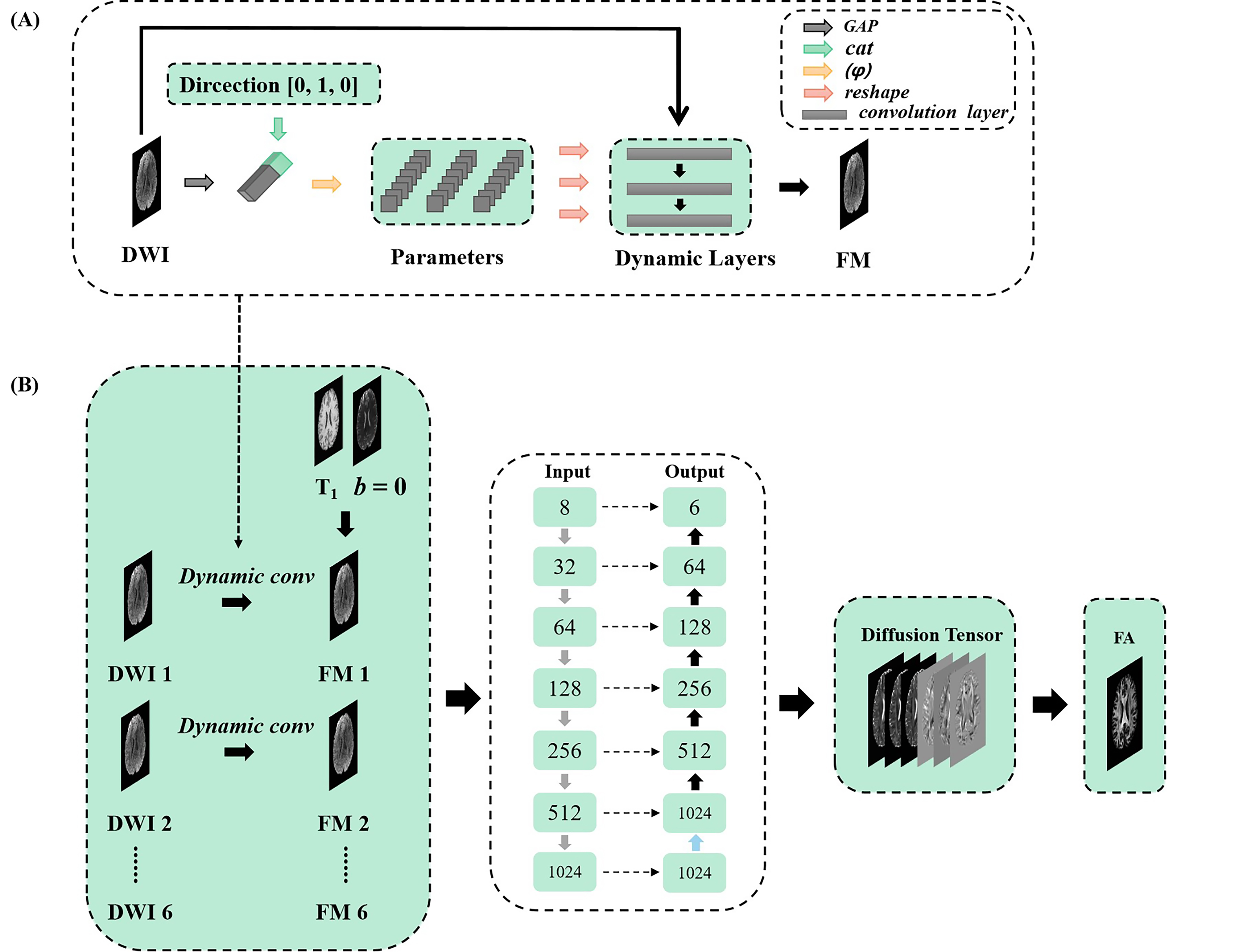
Figure 1. (A) The dynamic convolution kernel to achieve generalized reconstruction of DTI. The DWIs are aggregated into a one-dimensional vector via GAP concatenated with the diffusion direction vector. The concatenated vector is convolved and fully connected (φ) to get the kernel parameter, which are allocated to three dynamic convolution layers.
(B) Overall architecture of the proposed method for generalized reconstruction. The input of the network has one T1-weighted image, one b = 0 image, and six DWIs. The output of the network is diffusion tensor, which is used to fit the FA map.
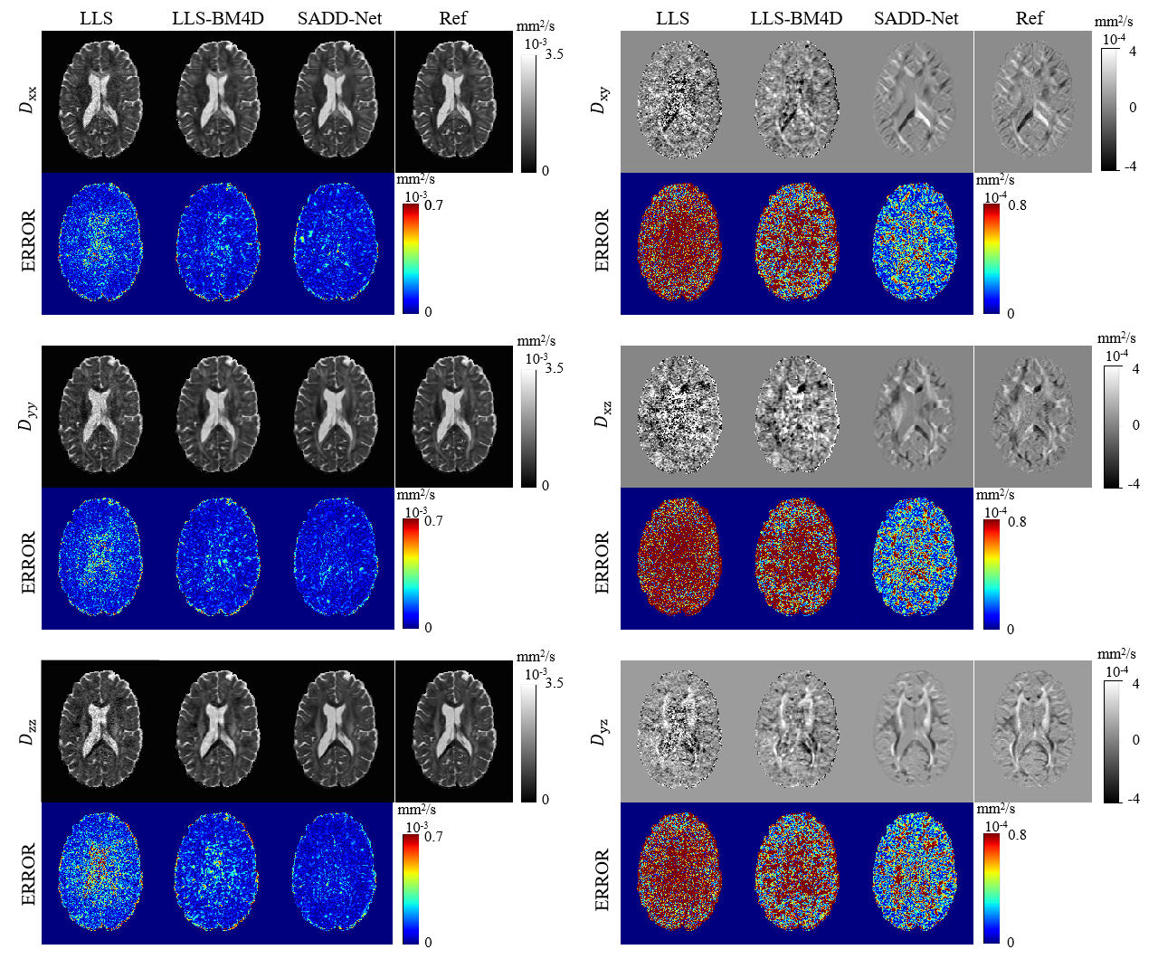
Figure 2. Comparison of 6
parameter maps of diffusion tensor reconstructed from least-squares fitting
(LLS), LLS after block-matching and 4D filtering (LLS-BM4D), and the proposed
method. The references were generated from LLS using 90 DWIs. Error maps
relative to the references were calculated.
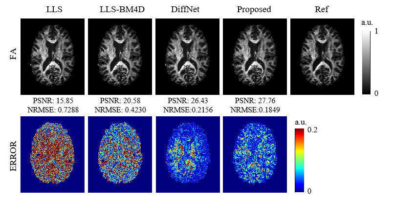
Figure 3. Comparison of FA
maps generated from LLS, LLS-BM4D, and DiffNet. The references were generated
from LLS using 90 DWIs. The PSNRs, NRMSEs, and error maps were calculated
relative to the reference.
DOI: https://doi.org/10.58530/2023/3110