Synopsis

Keywords: Image Reconstruction, Brain

MRI-Linac systems require real-time anatomical images with high geometric fidelity to localize and track tumours during radiotherapy treatments. Image distortions caused by B0 field inhomogeneity and slow MR acquisition hinder the application of real-time MRI-guided radiotherapy. Here, we develop and investigate a deep learning-based reconstruction pipeline to reconstruct B0 inhomogeneity distortion-corrected images (B0ReconNet) directly from k-space. MR acceleration techniques such as compressed sensing (CS) were integrated into B0ReconNet to further reduce acquisition time. Simulated and experimental data with fully sampled and retrospectively subsampled acquisitions on a 1T open bore MRI-Linac were used to validate the proposed method.

Introduction

MRI-Linac systems have been developed to enable accurate target localization and real-time tumour tracking for radiotherapy treatments [1]. The Australian 1T open bore MRI-Linac uses a split magnet design with a larger central gap (50cm) to facilitate patient positioning and treatment beam delivery [2]. However, the split bore structure compromises B0 field homogeneity, which causes image geometric distortions and potentially inaccurate dose delivery [3]. In addition, slow MR acquisition and reconstruction restrict the potential for real-time tumour tracking during radiotherapy treatments [4]. Our recently developed DCReconNet method shows deep neural networks have promises for fast and accurate image reconstruction with corrected gradient nonlinearity distortion [5]. In this work, we develop a deep learning network (B0ReconNet) to reconstruct B0 inhomogeneity distortion-corrected images directly from k-space domain. The compressed sensing (CS) technique was integrated into B0ReconNet to further reduce acquisition time. Simulated brain dataset and experimental distortion phantom images with fully sampled and retrospectively subsampled acquisitions on an MRI-Linac were used to validate the proposed method.

Method

Problem formulation
The forward gradient encoding process with B0 inhomogeneity can be formulated as [3, 6]: $$m\widetilde{F}s=b\qquad\qquad\qquad\qquad\qquad\qquad(1)$$ Where m is the undersampling matrix, b denotes the measured k-space signal, and s is the distortion-corrected image. $$$\widetilde{F}$$$represents the nonlinear Fourier transform matrix with the kernel of $$$\widetilde{e}=e^{-2\pi jk\widetilde{L}}$$$, where$$$\widetilde{L}$$$ is the distorted position caused by B0 inhomogeneity. The distorted position $$$\widetilde{L}$$$ can be found at the location $$$\widetilde{L}^{+}$$$ with a positive encoding gradient and $$$\widetilde{L}^{-}$$$ with a negative encoding gradient, governed by the equations [7] below: $$\widetilde{L}^{+}=L+\frac{dB_{0}(x,y,z)}{G_{L}} \qquad\qquad\qquad\qquad\qquad\qquad(2)$$ $$\widetilde{L}^{-}=L-\frac{dB_{0}(x,y,z)}{G_{L}} \qquad\qquad\qquad\qquad\qquad\qquad(3)$$ Where L is the undistorted position, $$$dB_{0}(x,y,z)$$$ is the B0 field deviation and $$$G_{L}$$$ is the applied gradient strength. The distortion-corrected image can be reconstructed by the penalized regression [4]:$$s=\mathop{\arg\min}_{s}\ \{\lambda P(s)+\|m\widetilde{F}s-b||_F^2\}\qquad\qquad\qquad\qquad\qquad\qquad(4)$$ Where P(s) represents a regularization function with a weighting parameter λ. Iterative regularisation algorithms can be used to solve Eq.(4), which however, have a high computational cost.
B0ReconNet
Recently, model-driven unrolling networks have shown promises in providing an accurate and rapid solution to MR reconstruction instead of using slow iterative algorithms. Unrolling networks incorporate known MR physics with well-defined interpretability. Based on an unrolling network architecture, Eq. (1) can be solved by the equation below [5]: $$s=\mathop{\arg\min}_{s}\ \{CNN(s)+\|m\widetilde{F}s-b||_F^2\}\qquad\qquad\qquad\qquad\qquad\qquad(5)$$ Where$$$\|m\widetilde{F}s-b||_F^2$$$ represents the data fidelity term, and a convolutional neural network CNN(s) was learned for effective regularizations. It is noted that $$$\widetilde{F}s$$$ represents a nonuniform Fourier transform operation, which can be calculated by Type-I Nonuniform Fast Fourier Transform (NUFFT).
Data preparation and network training
In this study, a 3D grid phantom with 3718 markers was scanned on the Australian 1T MRI-Linac system with positive and negative gradient encoding polarities to measure B0 inhomogeneity distortion. Based on the B0 measurement, a spherical harmonic expansion [8] was used to characterize the B0 field within the region of interest (ROI). 3000 T1-weighted brain images from a public MR dataset were used as training labels. Distorted brain images were simulated using Eq. (1) with acceleration factors (AF) of 2 and 4. Brain images were acquired from a whole-body MRI scanner, and the imaging parameters were: voxel size = 320 × 320 × 256, resolution = 0.7 mm × 0.7 mm × 0.7 mm, and TE/TR = 2.13 ms/2.4 s. The proposed B0ReconNet was based on the ISTA-Net architecture [8] and was trained on an Nvidia Tesla V100 GPU (32G) for 100 epochs (~10 hours) using these simulated brain images with Adam optimizer. Another 300 brain images from the same public MRI dataset were used to simulate testing data with AF=2 and AF=4. A 3D grid phantom was scanned from a 1T Australian MRI-Linac system with the imaging parameters: matrix size = 130 × 110 × 192, resolution = 1.8 mm × 2 mm × 1.8 mm, and TE/TR = 15 ms/5.1 s. Grid phantom data was retrospectively subsampled at AF=4.

Results

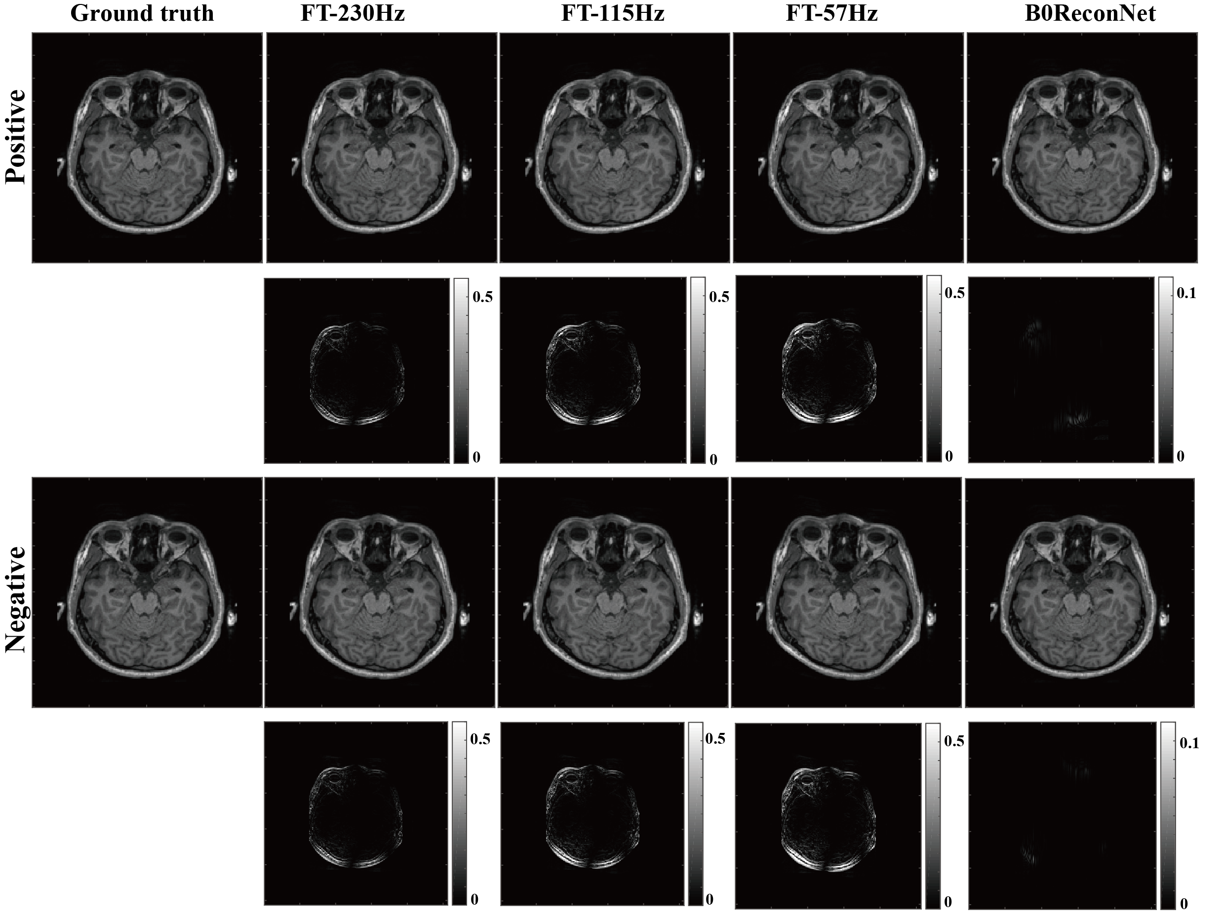
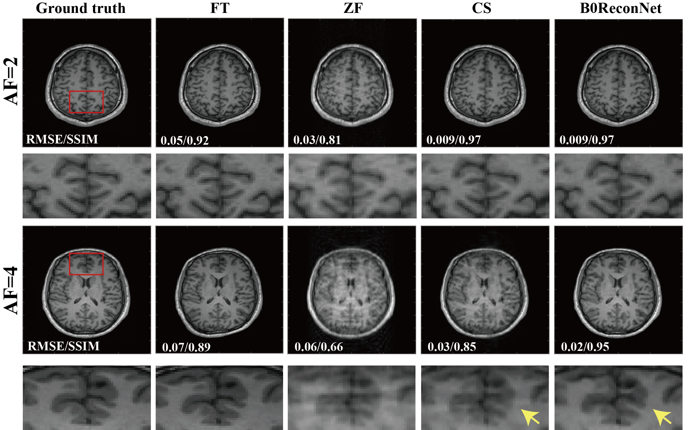
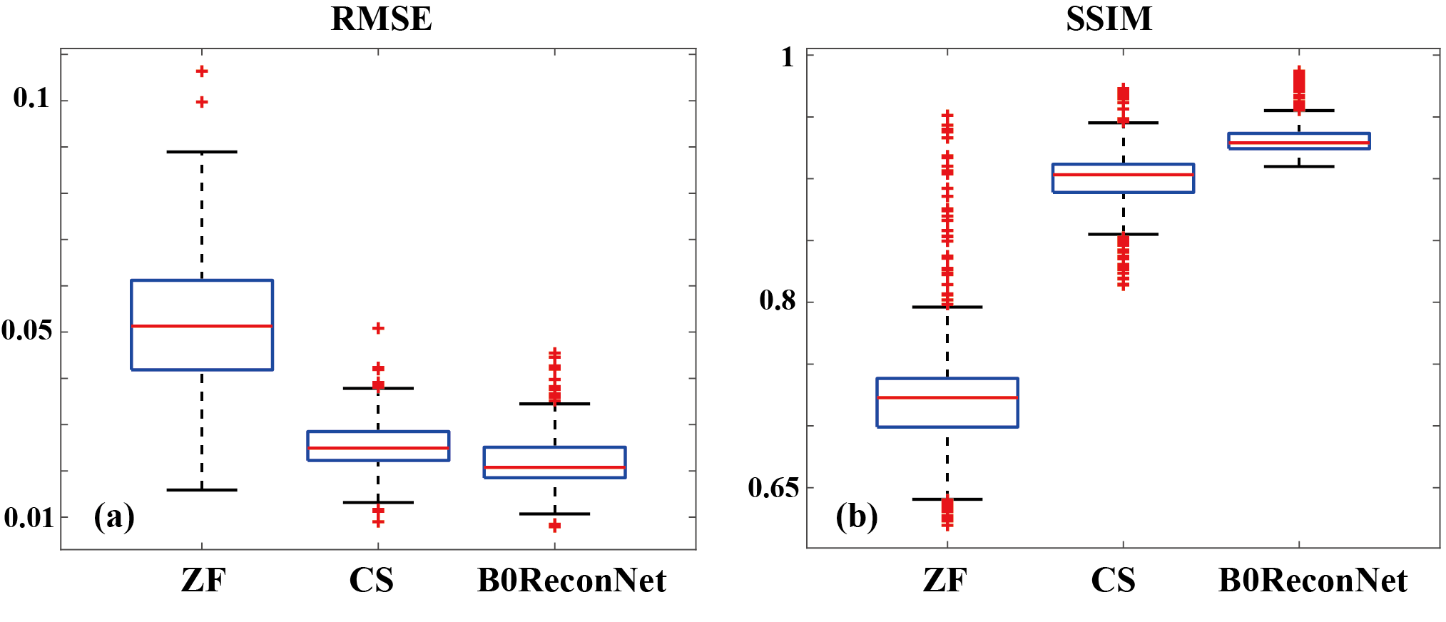
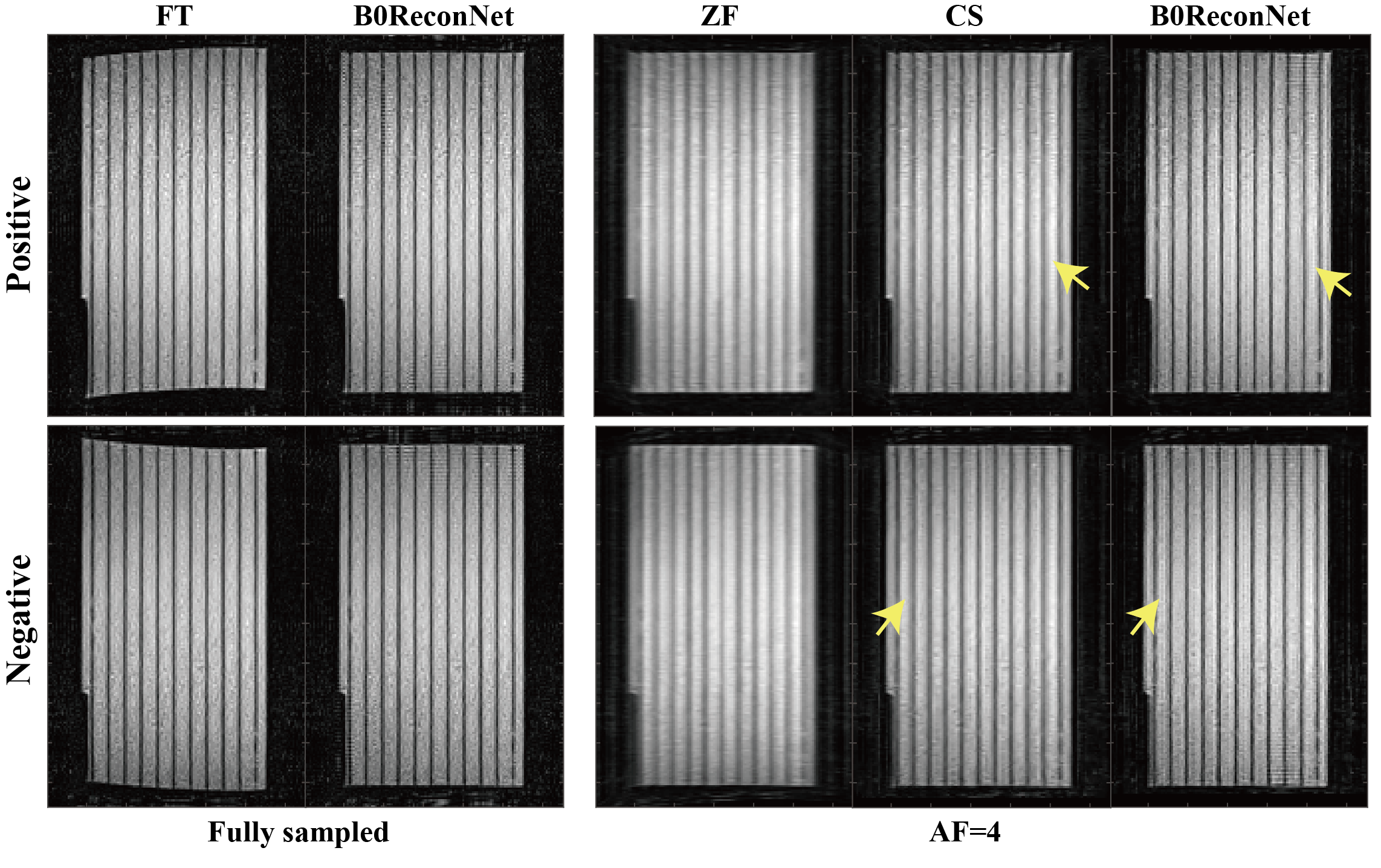
Fully sampled brain data with B0 inhomogeneity at different bandwidths is shown in Figure 1. Considerable geometric distortions were presented in conventional FT-reconstructed images, and more distortions resulted at lower bandwidth. By contrast, the B0ReconNet successfully reduced these distortions and resulted in minor errors (less than 10%), as indicated by the error maps. A subsampling mask with AF=2 and AF=4 was imposed on the B0 inhomogeneity-corrupted k-space data and then reconstructed by conventional CS-based regularization method, zero-filling method (ZF) and B0ReconNet. B0ReconNet achieved comparable results with the CS method at AF=2 with same root mean square error (RMSE) and structural similarity index (SSIM) values. While better structural details were preserved in the B0ReconNet-reconstructed images at AF=4, as indicated by yellow arrows. The RMSE and SSIM values were calculated on 300 testing simulated brain images at AF=4. As shown in Figure 3, the B0ReconNet provided the lowest RMSE and highest SSIM values compared with the other two methods. Experimental grid phantom results are shown in Figure 4. B0ReconNet resulted in better structural details than the CS and ZF methods. The inference time of B0ReconNet was 0.1s with GPU, making it feasible for real-time imaging applications.

Discussion and conclusion

Imaging results on simulated brain dataset and experimental phantom data demonstrated that the B0ReconNet enabled distortion-corrected image reconstruction from fully sampled and subsampled k-space data in real-time.

Acknowledgements

No acknowledgement found.