3088
Convergent and Interpretable Dynamic Cardiac MR Image Reconstruction with Neural Networks-based Convolutional Dictionary Learning1Physikalisch-Technische Bundesanstalt (PTB), Braunschweig and Berlin, Germany, 2Charité - Universitätsmedizin Berlin, Berlin, Germany, 3King’s College London, London, United Kingdom, 4Technical University of Berlin, Berlin, Germany, 5University of Innsbruck, Innsbruck, Austria
Synopsis
Keywords: Image Reconstruction, Machine Learning/Artificial Intelligence, Signal Processing, Sparsity-based Methods, Convolutional Dictionary Learning
In this work we consider three different variants physics-informed Neural Networks (PINNs) which use the convolutional dictionary learning framework for image reconsruction in dynamic cardiac MRI. Although all three NNs share the same mechanism for regularization, the iterative schemes differ because they are derived from different problem formulations. We compare the methdos in terms of reconstruction performance as well as stability with respect to the number of iterations. All three methods yield similarly accurate reconstructions. However, by construction, only one of the three methods defines a convergent reconstruction algorithm and is therefore stable w.r.t. to the number of iterations.Introduction
Physics-informed Neural Networks (PINNs) are typically constructed by unrolling reconstruction algorithms which are derived from specific problem formulations assuming fixed regularizers1. Depending on the specific problem formulation, one can derive PINNs with different theoretical properties regarding the interpretability and guarantees about the correctness of the obtained solutions2.For example, PINNs are often inherently linked to the number of iterations they were trained with. As a consequence, they are in general not guaranteed to yield convergent reconstruction algorithms.
In this work we construct three different PINNs using convolutional dictionary learning (CDL)3,4 as underlying regularization mechanism and illustrate the importance of using a convergent reconstruction algorithm when using PINNs.
Methods
In CDL, the image $$$\mathbf{x}$$$ is assumed to be generated from the convolution of unit-norm filters $$$\{d_k\}_k$$$ with corresponding sparse codes $$$\{\mathbf{s}_k\}_k$$$:$$ \mathbf{x} = \sum_{k=1}^{K} d_k \ast \mathbf{s}_k \hspace{1cm} \text{such that} \hspace{0.5cm} \| \mathbf{s}_k \|_1 \leq \alpha\hspace{0.5cm} \text{ for all } k. \hspace{3cm} (1)$$We now formulate three different problems which use the model (1) from which we can derive three different PINNs based on alternating minimization algorithms to learn the filters $$$\{d_k\}_k$$$ by back-propagation. Let $$$\mathbf{A}$$$ denote the MRI-operator and $$$\mathbf{y}:=\mathbf{A}\mathbf{x} + \mathbf{e}$$$ the measured $$$k$$$-space data, where $$$\mathbf{e}$$$ denotes Gaussian noise with standard deviation $$$\sigma>0$$$.
One possible approach5 is to relax the equality in (1) and include the constraints as penalty terms to obtain
$$\underset{\mathbf{x}, \{\mathbf{s}_k \}_k}{\min} \frac{1}{2}\|\mathbf{A} \mathbf{x} - \mathbf{y}\|_2^2 + \frac{\lambda}{2} \Big\| \mathbf{x} - \sum_{k=1}^K d_k \ast \mathbf{s}_k \Big\|_2^2 + \alpha \sum_{k=1}^K \| \mathbf{s}_k \|_1. \hspace{3cm} (2)$$
Since the variables $$$\mathbf{s}_k$$$ are coupled to the operator $$$\ast$$$ and the $$$\ell_1$$$-norm, solving the sub-problem with respect to $$$\{\mathbf{s}_k\}_k$$$ in (2) requires an iterative algorithm as ISTA6 or FISTA7 which needs to be run as many times as the algorithm alternates between the update of $$$\mathbf{x}$$$ and $$$\mathbf{s}_k$$$.
By the following formulation8 based on ADMM9 this can be avoided by re-formulating the sub-problem in the Fourier-domain and exploiting the closed-form solution given by the Sherman-Morrison formula9:
$$\underset{\mathbf{x}, \{\mathbf{s}_k \}_k, \{\mathbf{u}_k \}_k}{\min} \frac{1}{2}\|\mathbf{A} \mathbf{x} - \mathbf{y}\|_2^2 + \frac{\lambda}{2} \Big\| \mathbf{x} - \sum_{k=1}^K d_k \ast \mathbf{s}_k \Big\|_2^2 + \alpha \sum_{k=1}^K \| \mathbf{u}_k \|_1 \quad \text{s.t.} \quad \forall k: \mathbf{u}_k - \mathbf{s}_k = \mathbf{0}. \hspace{3cm} (3)$$
Problem (3) decouples all $$$\{\mathbf{s}_k\}_k$$$ from the $$$\ell_1$$$-norm at the cost of introducing new auxiliary varialbes $$$\{\mathbf{u}_k\}_k$$$ for which, however, the update is simple9.
Although the formulations in (2) and (3) are flexible in the sense that (1) is not strictly imposed on the image, the image update for (2) and (3) requires the use of an iterative solver, e.g. a conjugate gradient method (CG), which can be computationally demanding for large-scale problems.
As third alternative, we propose to explicitly make use of the model (1) and to unroll a sparse coding algorithm, similar as other works11,12. We set $$$\mathbf{x} := \sum_{k=1}^{K} d_k \,\ast \,\mathbf{s}_k$$$, $$$\mathbf{D}\mathbf{s}:=\sum_{k=1}^{K} d_k\, \ast\, \mathbf{s}_k$$$, $$$\mathbf{B}:=\mathbf{A} \mathbf{D}$$$ and formulate the reconstruction problem
$$\underset{\mathbf{s}}{\min} \frac{1}{2}\|\mathbf{B} \mathbf{s} - \mathbf{y}\|_2^2 + \alpha\|\mathbf{s}\|_1 \hspace{3cm} (4) $$
and unroll FISTA to obtain an approximate solution of (4), after which the image can be retrieved from (1).
We abbreviate the three different PINNs which are obtained by unrolling $$$T$$$ iterations of algorithms for solving (2), (3) and (4) by NN-CDL (CG + FISTA), NN-CDL (CG + ADMM)10 and NN-CDL (FISTA), respectively. Figure 1 shows an illustration of the NNs.
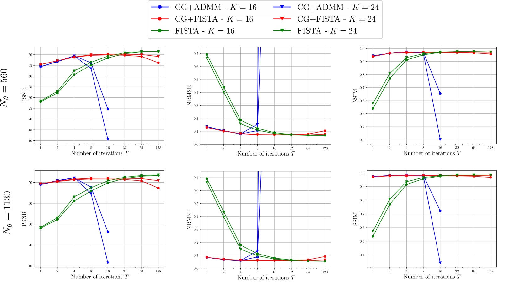
We compared the methods in terms of reconstruction performance and stability with respect to different $$$T$$$ used at test time on a non-Cartesian dynamic cardiac MRI problem. Our dataset consisted of 144/36/36 cardiac cine MR images which were used for training, validation and testing. We used $$$N_{\theta} = 560$$$ or $$$N_{\theta}=1130$$$ radial spokes and noise-level given by $$$\sigma=0.02$$$ for retrospectively generating input-target image-pairs.
For training, we used $$$T=4$$$, $$$T=5$$$ and $$$T=8$$$, i.e. the maximal number of iterations which were possible to use on a 48 GB GPU.
Results
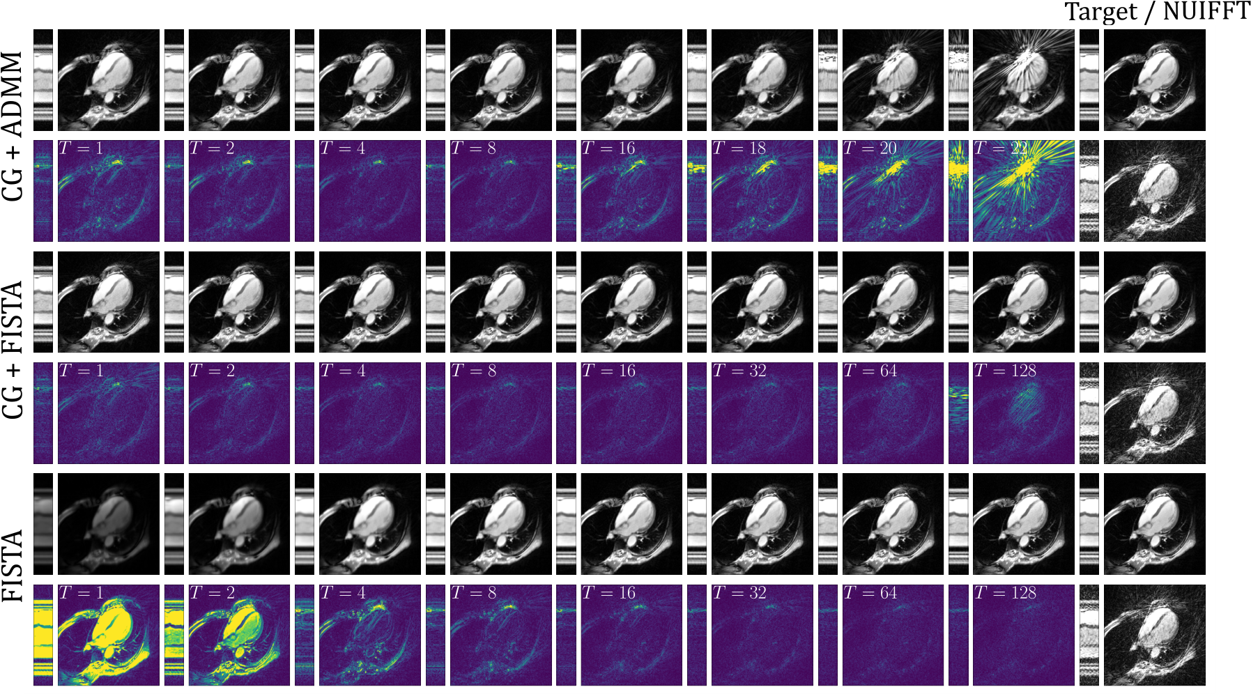
Figure 2 shows the average PSNR, NRMSE and SSIM13 obtained on the entire test-set for different $$$T$$$ used at test time. Figure 3 shows an example of reconstruction obtained with the different NNs. As can be seen, NN-CDL (CG+ADMM) is particularlry sensitive w.r.t. $$$T$$$, possibly due to the use of ADMM.Discussion
Although the results with the respective optimal number of iterations were comparable, NN-CDL (CG + ADMM) is the least stable with respect to $$$T$$$, followed by NN-CDL (CG + FISTA) which to some extent allows to vary $$$T$$$, followed by NN-CDL (FISTA) which is the most stable due to its convergence guarantees inherited from FISTA.In terms of training times, NN-CDL (CG + ADMM) is the fastest (~9 hours), possibly also because only $$$T=4$$$ could be used. Training NN-CDL (CG + FISTA) and NN-CDL (FISTA) takes longer (~1.5 / 3.5 days) as for each forward-pass, for FISTA, one must compute the operator-norms $$$\|\mathbf{D}\|_2$$$ and $$$\|\mathbf{A} \mathbf{D}\|_2$$$ with a power-iteration.
Conclusion
We have compared three different PINNs which use the CDL-model. We have seen that the problem formulation for deriving PINNs can have a large impact on the reconstruction algorithm. Although only shown for the CDL-model, we conjecture that same holds for other signal models as well. This work highlights the importance of convergence guarantees when applying reconstruction methods learned with PINNs.Acknowledgements
No acknowledgement found.References
1. Vishal Monga, Yuelong Li, and Yonina C Eldar. Algorithm unrolling: Interpretable, efficient deep learning for signal and image processing. IEEE Signal Processing Magazine, 38(2):18–44,2021.
2. Subhadip Mukherjee, Andreas Hauptmann, Ozan Öktem, Marcelo Pereyra and Carola-Bibiane Schönlieb (2022). Learned reconstruction methods with convergence guarantees. arXiv preprint arXiv:2206.05431.
3. Cristina Garcia-Cardona and Brendt Wohlberg. Convolutional dictionary learning: A comparative review and new algorithms. IEEE Transactions on Computational Imaging, 4(3):366–381,2018.
4. Il Yong Chun and Jeffrey A Fessler. Convolutional dictionary learning: Acceleration and convergence. IEEE Transactions on Image Processing, 27(4):1697–1712, 2017.
5. Tran Minh Quan and Won-Ki Jeong. Compressed sensing dynamic mri reconstruction using gpu-accelerated 3d convolutional sparse coding. In International conference on medical imagecomputing and computer-assisted intervention, pages 484–492. Springer, 2016.
6. Ingrid Daubechies, Michel Defrise, and Christine De Mol. An iterative thresholding algorithmfor linear inverse problems with a sparsity constraint. Communications on Pure and Applied Mathematics: A Journal Issued by the Courant Institute of Mathematical Sciences, 57(11):1413–1457, 2004.
7. Amir Beck and Marc Teboulle. A fast iterative shrinkage-thresholding algorithm for linear inverse problems. SIAM journal on imaging sciences, 2(1):183–202, 2009.
8. Brendt Wohlberg. Efficient algorithms for convolutional sparse representations. IEEE Transactions on Image Processing, 25(1):301–315, 2015.
9. Stephen Boyd, Neal Parikh, Eric Chu, Borja Peleato, Jonathan Eckstein. "Distributed optimization and statistical learning via the alternating direction method of multipliers." Foundations and Trends in Machine learning 3.1 (2011): 1-122.
10. Andreas Kofler, Christian Wald, Tobias Schaeffter, Markus Haltmeier, and Christoph Kolbitsch.Convolutional dictionary learning by end-to-end training of iterative neural networks. In Proceedings of European Signal Processing Conference (EUSIPCO) 2022.
11. Jian Zhang, and Bernard Ghanem. (2018). ISTA-Net: Interpretable optimization-inspired deep network for image compressive sensing. In Proceedings of the IEEE conference on computer vision and pattern recognition (pp. 1828-1837).
12. Jinxi Xiang, and Yonggui Dong, and Yunjie Yang.
(2021). FISTA-Net: Learning a fast iterative shrinkage thresholding
network for inverse problems in imaging. IEEE Transactions on Medical Imaging, 40(5), 1329-1339.
13. Zhou Wang, Alan C Bovik, Hamid RSheikh, and Eero PSimoncelli, (2004). Image quality assessment: from error
visibility to structural similarity. IEEE transactions on image processing, 13(4), 600-612.
Figures
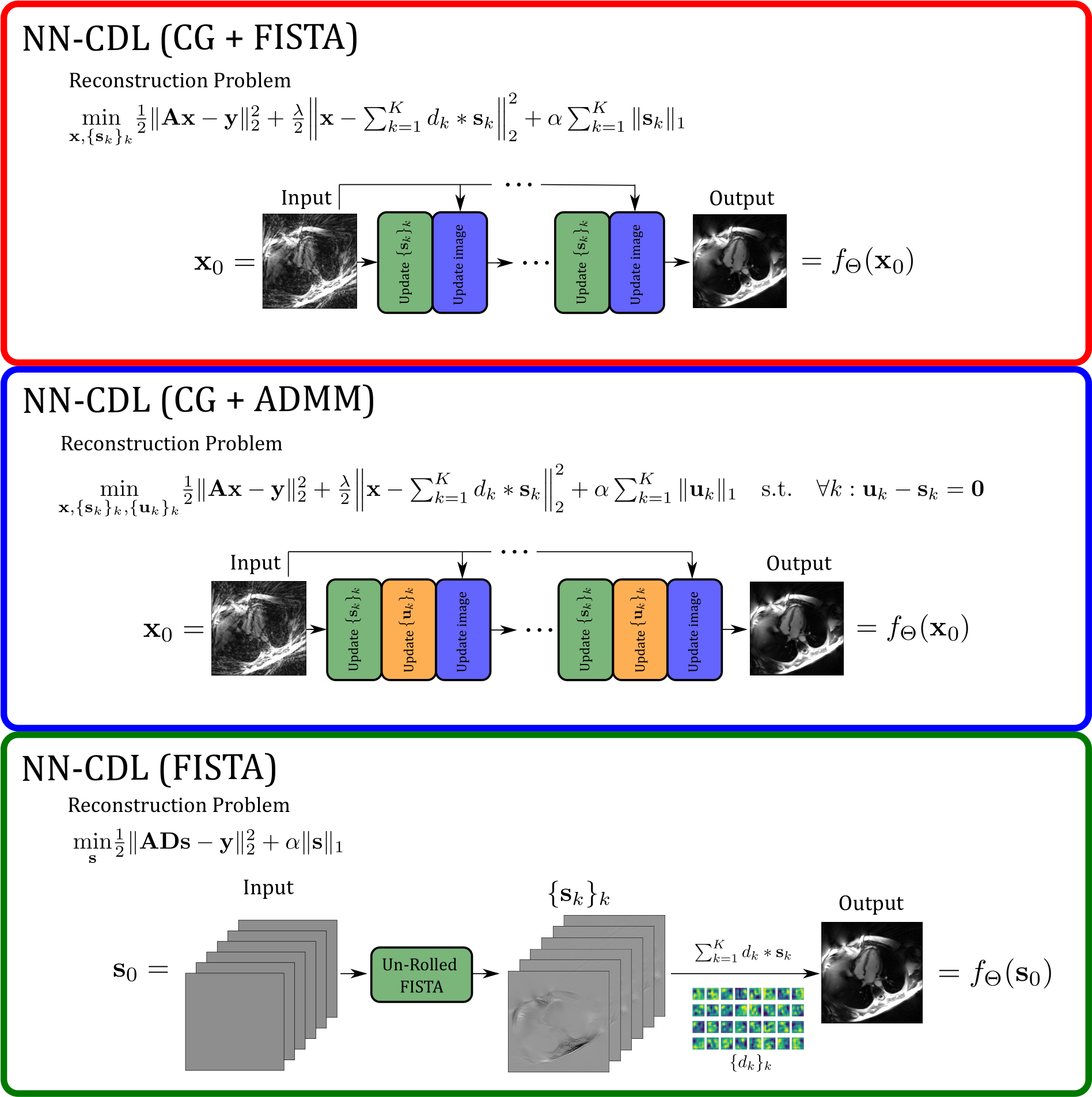
Figure 1: The three different NNs based on the CDL model (1). In NN-CDL (CG+FISTA) and NN-CDL (CG-ADMM), the CDL-regularization is only approximately imposed employing a quadratic penalty term which is weighted by $$$\frac{\lambda}{2}$$$ and alternating minimization-based algorithms are used to reconstruct the image. NN-CDL (FISTA), in contrast, explicitly uses the model (1) and un-rolls $$$T$$$ iterations to directly obtain an estimate of the sparse codes which can then be used to generate the image according to (1).