3046
When texture does not matter: Misinterpretation of deep learning-based Alzheimer's disease classification1Medical University of Graz, Graz, Austria
Synopsis
Keywords: Alzheimer's Disease, Machine Learning/Artificial Intelligence
Recent studies have shown Clever Hans effects in e.g. a widely used MRI tumor dataset. Clever Hans was a horse in the early 20th century that could supposedly do some arithmetic, although it only reacted to unintended cues of its owner. Inspired by these insights, we used T1w images from the ADNI database and removed the texture using threshold binarization. By using a standard deep neural network we separated images from Alzheimer's patients (n=404) from normal controls (n=905). This study revealed that volumetric measures are overwhelmingly relevant for the classification, while textures (T1w-contrast variations) are neglectable.Introduction
Deep convolutional neural networks (CNNs) can learn features from MRI for the classification of neurological disorders such as e.g. Alzheimer's disease (AD) 1. However, CNNs are mainly considered as black boxes, which lack interpretability by humans 2. Recent work in a widely used MRI tumor dataset revealed an underlying Clever Hans bias coming from the strategic location of specific tumor types 3. Previous work on AD classification 4 showed that (a) texture and/or (b) volumetric features might be relevant for the classification outcome, but could not definitely determine the individual contributions of the aforementioned factors.Therefore, here we used T1w data from the ADNI database (https://adni.loni.usc.edu) in a conventional 3D subject level CNN. To rule out the contribution of texture we trained the CNNs with both, native T1w and binarized images and additionally investigated the impact of skull stripping.
Methodology
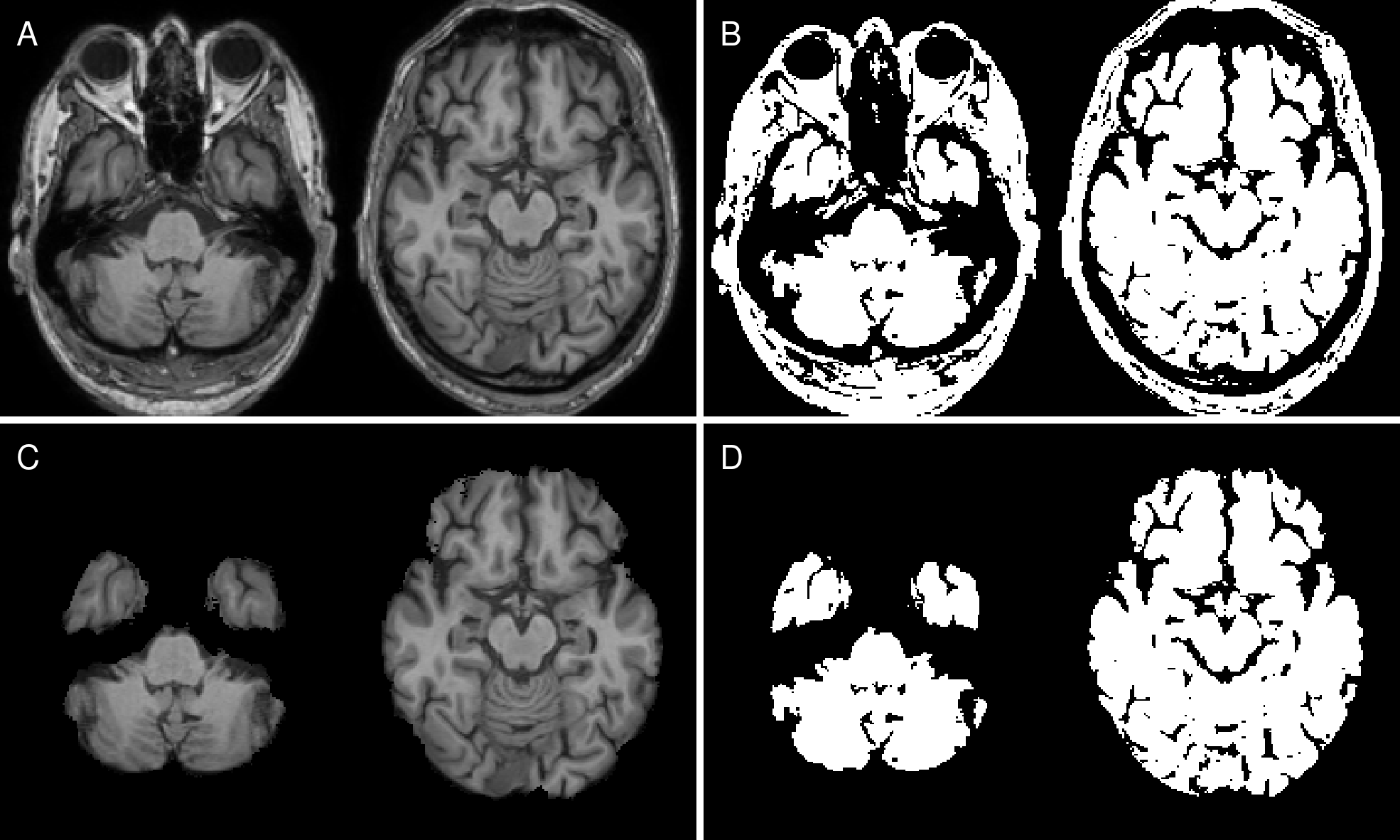
Dataset. We retrospectively selected 404 MRI datasets from 135 patients with probable AD (mean age=75.4±7.8 years) and 905 MRIs from 220 age-matched normal controls (mean age=75.6±6.7 years) from the ADNI database. Patients and controls were scanned using a consistent MRI protocol at 3 Tesla (Philips Medical Systems) including a T1-weighted MPRAGE sequence (1.0x1.0x1.2mm³, TR/TE=6.8/3.2ms, FA=9°). AD and NC data were sampled into training, validation and test sets (ratio 70:15:15), while maintaining all scans from one person in the same set. To ensure the same class distribution in all setups, final sets were created by combining one set from each cohort. The sampling procedure was repeated 10 times to enable a bootstrapping analysis.Preprocessing. T1-weighted images were reoriented to standard space using FSL-REORIENT2STD, cropped to 160x240x256 matrix size and bias field corrected using N4BiasFieldCorrection 5. Brain masks from each T1-weighted image were obtained using SIENAX from FSL 6. T1-weighted images were registered nonlinearly using FSL-FNIRT 7 to the MNI152 template. Following registration, we binarized the T1-weighted images using a manually chosen threshold of 27.5% of the maximum intensity to create binary masks, which only preserved shape information (Figure 1).
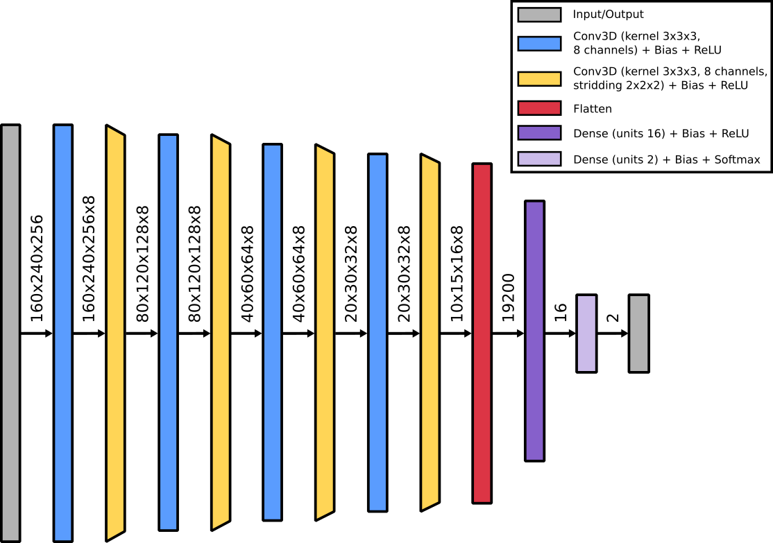
Standard classification network. We utilize a standard classifier network, which uses the combination of a single convolutional layer followed by a down-convolutional layer as the main building block. The overall network stacks four of those main building blocks before passing the data through two fully connected layers. Each layer is followed by a Rectified Linear Unit (ReLU) nonlinearity, except for the output layer where a Softmax activation is applied (cf. Figure 2 for details).
Network weights initialization. To ensure the same starting point for the network training, we created 3 network weights initializations. Network training with a given data sampling was repeated for all network weights initializations.
Training. We trained models with input images nonlinearly registered to MNI152 space, with/without skull-stripping, and with/without binarization. Each model was trained using Adam 8 for 60 epochs with a batch size of 6.
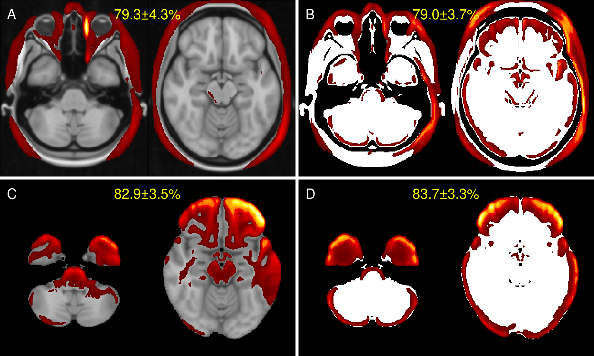
Heat mapping. Heat maps were created based on the deep Taylor decomposition (DTD) method described in 9.
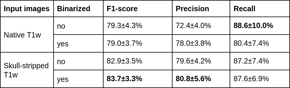
Bootstrapping analysis. For each data sampling (10 data samplings) and for each network weights initialization (3 weights initializations) we repeated the training of the network, creating overall 30 training sessions with the same input image configuration 10. Training sessions that did not converge (e.g. loss remained the same) were excluded from further analysis in all setups. Because the classes in the data set were unbalanced we report the mean performance and standard deviation of F1-score, precision and recall 11. Mean heat maps were created from all test images of all included training sessions.
Results
Figure 3 summarizes the precision and recall as well as the harmonic mean performance (F1-score) for the bootstrapping setup of all configurations (with/without skull stripping; with/without binarization). Mean heat maps for classification decisions on training data sets of all data samplings for all included models are shown in Figure 4. Qualitatively, the mean heatmaps from inputs with binarization show a substantial overlap with the results from inputs without binarization.Discussion and Conclusion
Previous studies using T1-weighted MRIs could not definitively conclude whether volumetric features, signal intensity changes or other factors are relevant for the CNN-based classification of AD 4,12. Clever Hans effects have been recently found in 13 as well as in a widely utilized MRI brain tumor dataset 3. Here, we set out to investigate the mechanisms underlying CNN-based classification in a highly representative AD dataset from ADNI. The present study was specifically designed to rule out relevant effects of T1w texture by binarizing the T1w input images.In conclusion, we revealed a Clever Hans effect learned by deep learning in a widely utilized AD dataset. Deep learning AD classification based on conventional T1w MR images is strongly driven by volumetric features, whereas texture induced by T1w contrast variations does not improve classification performance. Further work is warranted in other AD datasets as well as in other neurological disorders where atrophy as a consequence of neurodegeneration plays a major role.
Acknowledgements
This study was funded by the Austrian Science Fund (FWF grant numbers: P30134, P35887). This research was supported by NVIDIA GPU hardware grants.References
1. Wen J, Thibeau-Sutre E, Diaz-Melo M, et al. Convolutional neural networks for classification of Alzheimer’s disease: Overview and reproducible evaluation. Med Image Anal. 2020;63:101694. doi:10.1016/j.media.2020.101694
2. Samek W, Binder A, Montavon G, Lapuschkin S, Muller KR. Evaluating the Visualization of What a Deep Neural Network Has Learned. IEEE Trans Neural Netw Learn Syst. 2017;28(11):2660-2673. doi:10.1109/TNNLS.2016.2599820
3. Wallis D, Buvat I. Clever Hans effect found in a widely used brain tumour MRI dataset. Medical Image Analysis. 2022;77:102368. doi:10.1016/j.media.2022.102368
4. Tinauer C, Heber S, Pirpamer L, et al. Explainable Brain Disease Classification and Relevance-Guided Deep Learning.; 2021:2021.09.09.21263013. doi:10.1101/2021.09.09.21263013
5. Tustison NJ, Avants BB, Cook PA, et al. N4ITK: improved N3 bias correction. IEEE Trans Med Imaging. 2010;29(6):1310-1320. doi:10.1109/TMI.2010.2046908
6. Smith SM, Zhang Y, Jenkinson M, et al. Accurate, robust, and automated longitudinal and cross-sectional brain change analysis. Neuroimage. 2002;17(1):479-489. doi:10.1006/nimg.2002.1040
7. Non-linear registration aka spatial normalisation FMRIB Technial report TR07JA2. – ScienceOpen. Accessed November 9, 2022. https://www.scienceopen.com/book?vid=13f3b9a9-6e99-4ae7-bea2-c1bf0af8ca6e
8. Kingma DP, Ba J. Adam: A Method for Stochastic Optimization. In: Bengio Y, LeCun Y, eds. 3rd International Conference on Learning Representations, ICLR 2015, San Diego, CA, USA, May 7-9, 2015, Conference Track Proceedings. ; 2015. Accessed November 10, 2021. http://arxiv.org/abs/1412.6980
9. Montavon G, Lapuschkin S, Binder A, Samek W, Müller KR. Explaining nonlinear classification decisions with deep Taylor decomposition. Pattern Recognition. 2017;65:211-222. doi:10.1016/j.patcog.2016.11.008
10. Bouthillier X, Delaunay P, Bronzi M, et al. Accounting for Variance in Machine Learning Benchmarks. arXiv:210303098 [cs, stat]. Published online March 1, 2021. Accessed December 1, 2021. http://arxiv.org/abs/2103.03098
11. Saito T, Rehmsmeier M. The Precision-Recall Plot Is More Informative than the ROC Plot When Evaluating Binary Classifiers on Imbalanced Datasets. PLOS ONE. 2015;10(3):e0118432. doi:10.1371/journal.pone.0118432
12. Böhle M, Eitel F, Weygandt M, Ritter K. Layer-Wise Relevance Propagation for Explaining Deep Neural Network Decisions in MRI-Based Alzheimer’s Disease Classification. Front Aging Neurosci. 2019;11:194. doi:10.3389/fnagi.2019.00194
13. Lapuschkin S, Wäldchen S, Binder A, Montavon G, Samek W, Müller KR. Unmasking Clever Hans predictors and assessing what machines really learn. Nat Commun. 2019;10(1):1096. doi:10.1038/s41467-019-08987-4
Figures