Synopsis

Keywords: CEST & MT, Machine Learning/Artificial Intelligence

Here we introduced a model-based deep learning approach which enabled joint optimization of both sampling and reconstruction for CEST MRI. The main purpose is to investigate an efficient undersampling pattern for CEST acceleration. Retrospective results (4X) showed that the proposed workflow is capable of leveraging redundancy information from optimized sampling pattern, further reconstructing gold-standard-consistent contrast maps.

Introduction

Chemical exchange saturation transfer is a MR contrast mechanism that can review promising metabolic information for various clinical applications. In order to overcome the obstacles resulted from long scan time, fast acquisition and reconstruction strategies are in critical needs for CEST clinical applications^[1][2][3]. However, the under-sampling pattern suitable for CEST remains to be explored. To investigate an efficient undersampling pattern for CEST acceleration, we introduced a model-based^[4][5] deep learning approach which enabled a joint optimization of CEST sampling and reconstruction.

Methods

Parameterization of Sampling Pattern
We represent the forward model as:
$$\mathrm{b}=A_{k, \Delta \omega} X=F_{k, \Delta \omega} S X$$
where $$$F_{k, \Delta \omega}$$$ is Fourier transformation and S is multi-channel sensitivity maps. Since the transformation parameter k in fast Fourier transformation is discrete and non-differentiable, we build a Fourier transform matrix with an one-dimensional parameters k1 to km, where m is the number sampling locations. The matrix can be expressed as $$$F(k, r)=e^{-j k r}$$$, which maps the spatial locations to continuous domain Fourier samples. In order to ensure the difference of the sampling locations of different offsets and further leverage redundancies, each offset has a set of parameters that determine the sampling locations:
$$F_{k, \Delta \omega}=\left\{F_{k, \Delta \omega 1}, F_{k, \Delta \omega 2}, \cdots, F_{k, \Delta \omega n}\right\}$$
Data Acquisition & Preprocessing
14 healthy volunteers were scanned on a Philips 3T scanner (Ingenia CX 3.0T; Philips Medical Systems, Best, The Netherlands), using a body coil for transmission and a 32-channel head coil for reception. All subjects signed the written informed consent. The CEST sequence used a saturation duration of 2 seconds and power of 1 uT, followed by TSE readouts (TSE factor=174). In total 32 saturation offsets were collected for Z-spectra fitting, distributed from -10 ppm to 10ppm. Other scan parameters are: FOV=230×201×60 mm3, spatial resolution=1.8×1.8×3 mm3, TR/TE=3.39 s/7.8 ms.
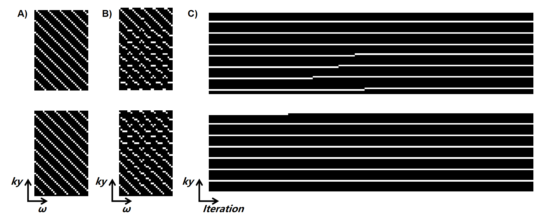
In terms of data preprocessing, both training and testing data were normalized. Sensitivity maps were estimated by ESPIRIT. Initial sampling pattern is shown in Figure 2(A). Each offset has a 28x1 trainable sampling location parameters, which is equivalent to 4X undersampling.
Network Training
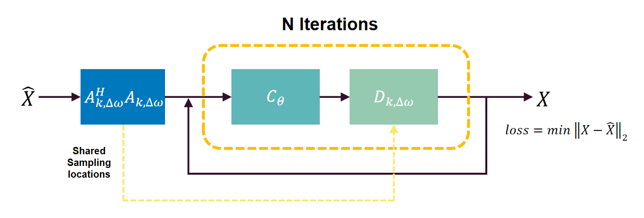
Figure 1 shows the proposed deep learning framework. The framework alternates between data consistency layer $$$D_{k, \omega}$$$ and CNN denoiser $$$C_{\theta}$$$:
$$\begin{array}{c}x_{n+1}=\left(A^{H} A+I\right)^{-1}\left(z_{n}+A^{H} A \widehat{X}\right) \\z_{n+1}=C_{\theta}\left(x_{n+1}\right)\end{array}$$
where $$$\widehat{x}$$$ denotes fully-sampled complex image. We unrolled the network for N iterations to solve:
$$\mathrm{X}_{\text {recon }}=\operatorname{argmin}_{\mathrm{X}}\left\|\mathrm{A} \widehat{\mathrm{X}}-F_{k, \Delta \omega} S X\right\|_{2}^{2}+\left\|\mathrm{X}-C_{\theta}(X)\right\|_{\mathrm{F}}^{2}$$
In terms of implementation details, the CNN denoiser was implemented as a 4-layer U-net with 3x3 trainable filters. The data consistency layer were implemented using a conjugate gradient algorithm. All parameters were optimized by an Adam optimizer to minimize a mean squared error (MSE) loss:
$$\operatorname{argmin}_{\theta, k}\left\|D_{k, \Delta \omega}\left(C_{\theta}\left(A^{H} A \widehat{X}\right)\right)-\widehat{X}\right\|_{2}^{2}$$
In training step, denoiser weight and sampling locations were simultaneously updated. After training, both denoiser and sampling mask were fixed for inference. Note that sampling locations in k-space center were frozen. In our preliminary experiment, iteration number N was set to 1. The network was based on Tensorflow 2.4.0 and was trained for 500 epochs on a RTX3060 12G GPU, taking about 26 hours.

Results and Discussion

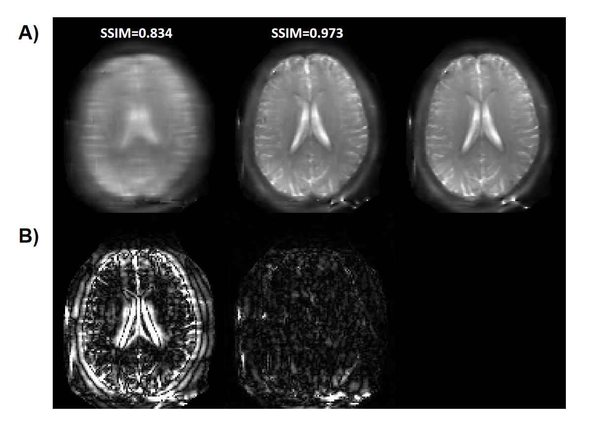
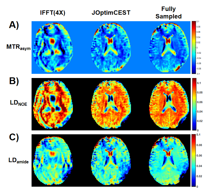
Figure 2(B) and (C) depicted the optimized sampling locations. As training, the sampling locations of each offset were automatically optimized to improve acquisition efficiency. After the network converged, the optimized sampling pattern and the reconstruction network were obtained simultaneously.
Figure 3 compared the saturation-weighted images at 3.5 ppm obtained from the zero-filling data, reconstructed data from the optimized undersampled measurement and fully sampled data. The difference between reconstructed images and fully-sampled golden standard suggested the good recovery of anatomy structure. The metrics of joint optimized test data achieved 37.67 dB of PSNR, 0.985 of SSIM, and 6.73e-4 of nMSE, which declared a good performance of joint optimization approach. We further calculated the contrast maps through the widely-used quantification methods, i.e., MTR asymmetry and Lorentzian difference (LD) (Figure 4), which indicted the retrospective results were consistent with fully sampled results. At present, we set the initial sampling mask as a uniform one, and the loss function is a trivial MSE loss. In order to make sampling pattern conductive to accurate contrast maps (e.g. more k-space center data for ±3.5ppm), CEST-related loss function and constraint remain to be investigated.

Conclusion

In this study, we initially validated the joint optimization of sampling pattern and reconstruction for CEST imaging using an unrolled deep-learning approach. The results suggested that the proposed workflow can automatically find efficient sample locations and reconstruct similar quality images as the fully-sampled image, which may help clinical promotion of CEST imaging.

Acknowledgements

This work was supported by the National Natural Science Foundation of China [grant numbers 82071914］