Synopsis

Keywords: Machine Learning/Artificial Intelligence, Machine Learning/Artificial Intelligence, unsuperivised learning

Existing supervised deep learning methods for quantitative susceptibility mapping (QSM) could lead to degraded results when applied to phase images acquired with different scan parameters, such as image resolution and acquisition orientation. This work proposes a novel unsupervised learning method incorporating style transfer and deep image prior to enabling the reconstruction of susceptibility maps from local field maps acquired with any scan parameters. To speed up the inference, a pre-training strategy is also proposed, reducing reconstruction time from minutes to seconds.

Introduction

Quantitative susceptibility mapping (QSM) reconstructs magnetic susceptibility distribution from gradient-echo phase maps. The final step of the QSM pipeline requires solving an ill-posed dipole. Numerous methods based on optimization and deep learning have been proposed, most of which are limited by time-consuming parameter tuning and poor model generalizability. Deep Image Prior [1] (DIP) demonstrates that convolutional neural networks (CNNs) can potentially model the ill-posed inversion process with the network serving as a prior for regularization. Inspired by DIP, we propose an unsupervised deep learning method for QSM reconstruction without the need for paired data. Besides, a pre-training autoencoder and a style transfer mechanism [2] are also adopted to further speed up and enhance the reconstruction.

Methods

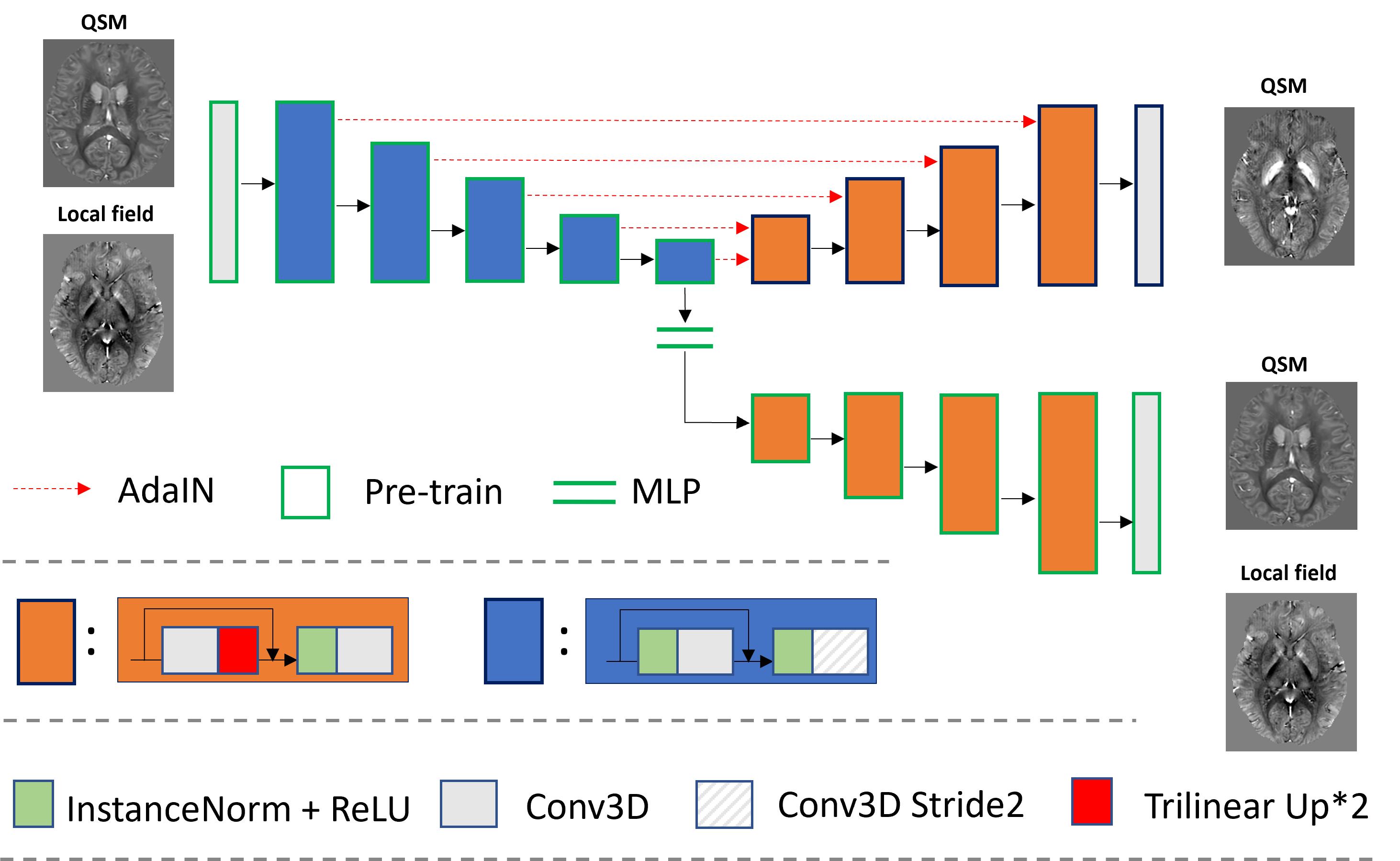
The proposed method aims to reconstruct the susceptibility maps while suppressing streaking artifacts due to noise and errors in in-vivo acquisitions. As shown in the original DIP paper, these out-of-distribution noise and errors require more training epochs than the underlying images for CNNs to represent, hence CNNs serve as a deep image prior to regularizing the reconstruction result. Here, we build a unique encoder-decoder network architecture that comprises one encoder and two decoders. As illustrated in Figure 1, the encoder and the upper decoder with skip connections output susceptibility maps. The encoder and the lower decoder form an Auto-Encoder structure, which is pre-trained using 96 full-sized brain local field and susceptibility maps of 1 mm3 resolution in pure axial head orientation. Then for each skip connection between the encoder and the upper decoder and the bottom bottleneck connection, an Adaptive Instance Normalization (AdaIN) operation is applied to transfer the local field style feature maps to the QSM style in real-time:
$$\begin{matrix} {AdaIN\left( {x,~y} \right) = ~\frac{\left( {x - ~\mu_{x}} \right)}{\sigma_{x}}*~\sigma_{y} + ~\mu_{y},~(1)} \\ \end{matrix}$$
where x and y are feature maps from local field and susceptibility maps respectively, μ and σ are the corresponding mean and standard deviation.
To optimize the real-time inference, A style loss similar to [2] as well as the QSM model loss were optimized to train the network in an unsupervised manner:
$$\begin{matrix} {{L = L_{model} + L}_{style},~(2)} \\ \end{matrix}$$
$$\begin{matrix} {L_{style} = {\sum\limits_{i}^{4}\left( {\mu_{\zeta_{i}{(\overset{-}{y})}} - \mu_{\zeta_{i}{(y)}}} \right)^{2}} + \left( {\sigma_{\zeta_{i}{(\overset{-}{y})}} - \sigma_{\zeta_{i}{(y)}}} \right)^{2},~(3)} \\ \end{matrix}$$
$$\begin{matrix} {L_{model} = \left( {F^{- 1}DF\overset{-}{y} - x} \right),~(4)} \\ \end{matrix}$$
where denotes the ith encoding block in the encoder, F the Fourier transform and D the magnetic dipole, the final prediction. During inference time, the pre-trained encoder is fixed, while the upper decoder network gets updated minimizing the total loss term in Eq. (2).

Results

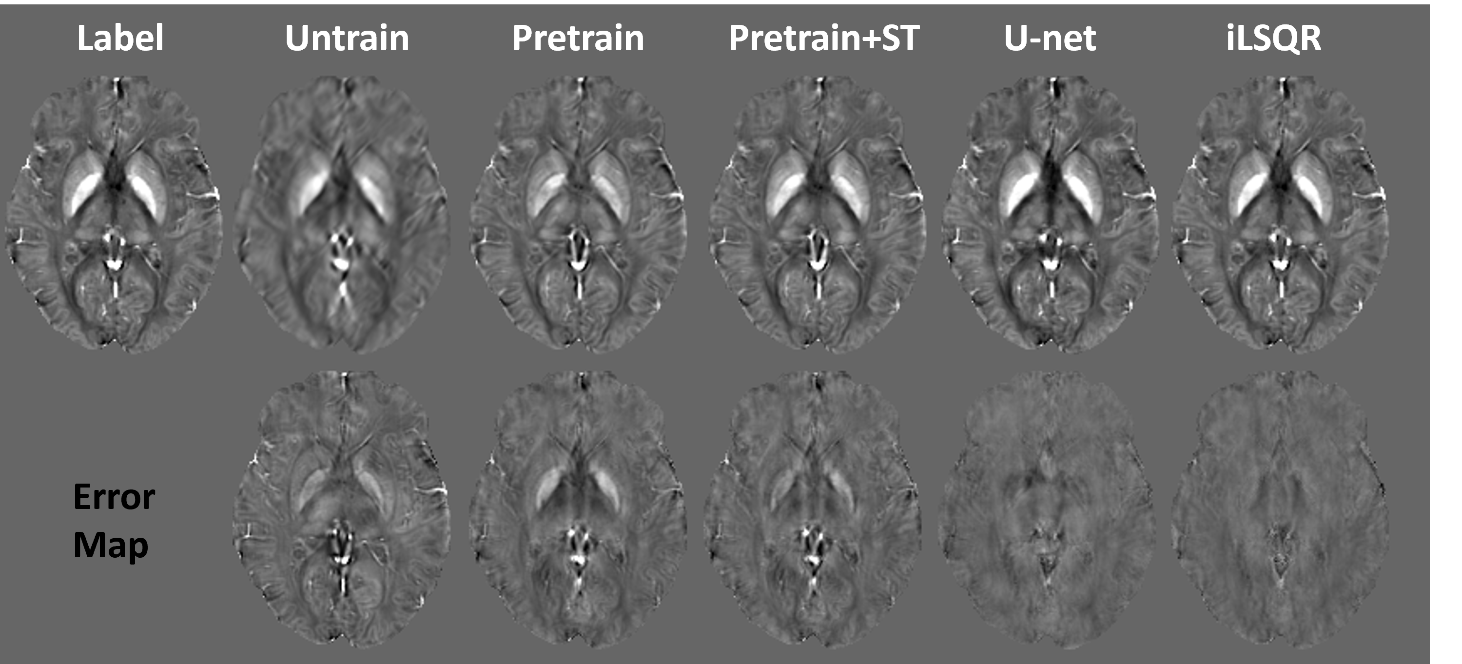
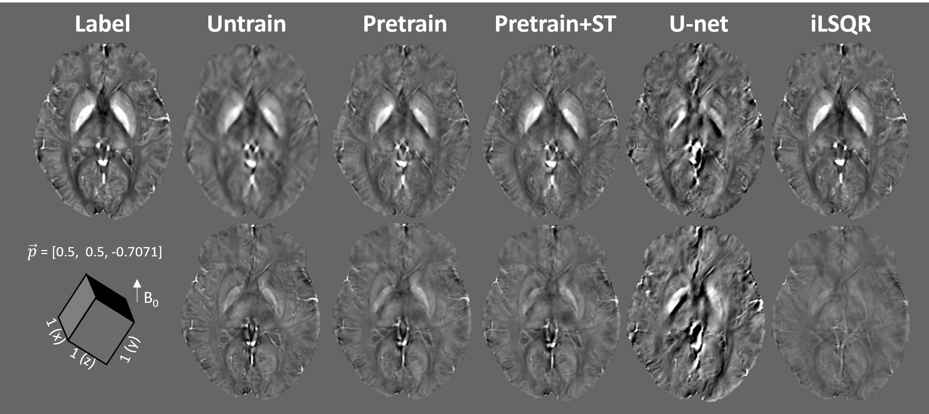
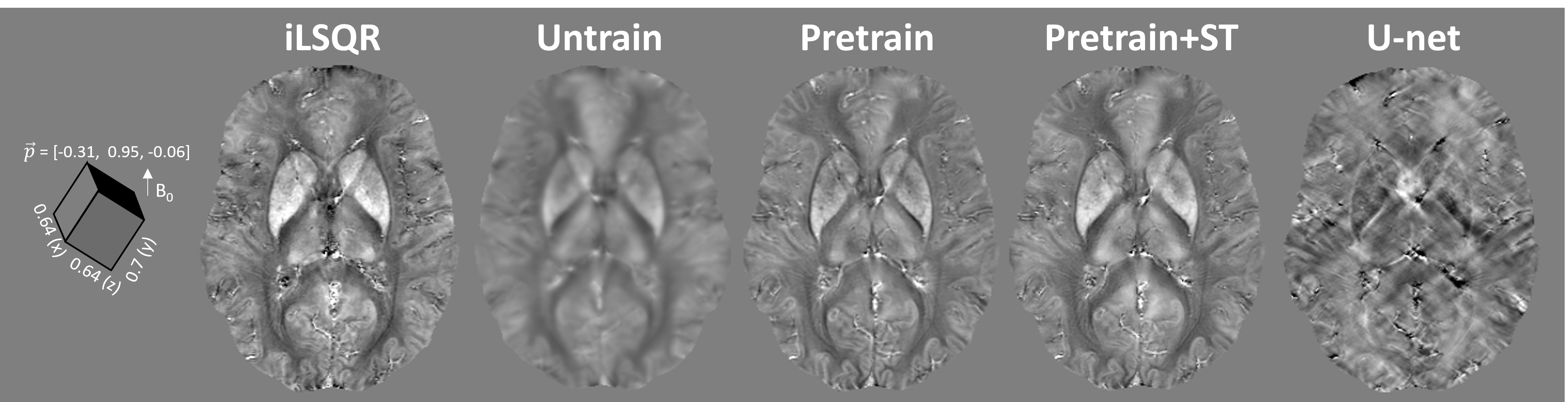
An ablation study in Figure 2 was demonstrated on a simulated brain volume with vox = [1, 1, 1] mm³ and acquisition orientation H = [0, 0, 1]. It is shown that with the same number of epochs, pre-training the encoder significantly improved the results, which was further enhanced by adding the style transfer. Another simulation with the oblique acquisition (H = [0.5, 0.5, 0.7071]) was shown in Figure 3. The supervised U-net [3, 4] trained on pure axial orientation failed to reconstruct QSM in this case, while the proposed unsupervised methods successfully resolved the oblique dipole kernel, with pre-train + style transfer (ST) performed the best. Figure 4 showed an in-vivo experiment, with acquisition parameters of (vox = [0.64, 0.64, 0.70] mm³, H = [-0.31, 0.95, -0.06]). A similar conclusion can be drawn that the unsupervised approach substantially improved generalizability than the supervised Unet. Moreover, the proposed method led to QSM image with reduced noise and artifacts compared to the conventional iLSQR [5] method, due to the deep image prior regularization of the neural network.

Discussion

The proposed method significantly shortened the inference time by pre-training the encoder. Moreover, the addition of style transfer alleviated susceptibility contrast suppression and improved the accuracy of the QSM reconstruction in the pure-axial case (Fig. 2). However, the proposed style transfer demonstrated less improvement in the oblique case (Fig. 3), which may be because only pure-axial data were used in the pretrain stage of the encoder for style extraction. The proposed method still underestimated the susceptibility map compared to iLSQ and U-net (Fig. 2), but on the other hand, obtained the improved generalizability to solve the dipole inversion in the anisotropic and oblique acquisition case.

Acknowledgements

HS received funding from Australian Research Council (DE210101297).