Synopsis

Keywords: Image Reconstruction, Data Processing, Image super-resolution, model bias, deep learning

Deep Learning based image super-resolution methods are biased towards training data modeling. Generalizability of DL based super-resolution frameworks can be improved by introducing variability and diversity in the training data.

Introduction

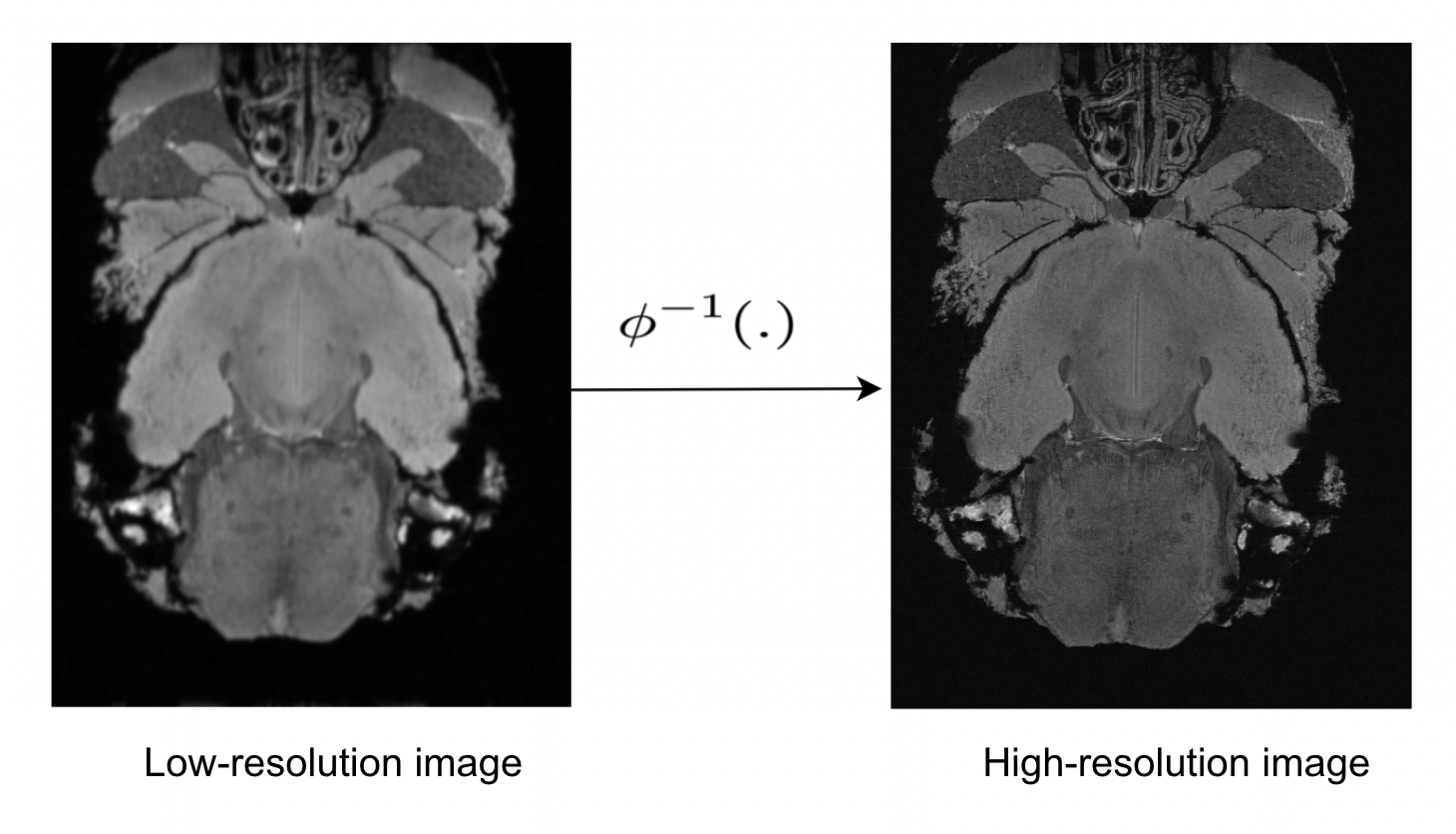
Deep learning-based methods have been the preferred choice for solving various learning problems such as image super-resolution ¹ and reconstruction in the field of medical imaging. In image super-resolution, the goal is to estimate the high-resolution image from the given low-resolution image. The image super-resolution problem can be formulated as:
$$ \textbf{y} = \phi ( \textbf{x}; \theta_{d}),$$
where $$$\phi$$$ is the degradation model with parameter $$$\theta_{d}$$$ that a desired high-resolution image $$$\textbf{x}$$$ undergoes and $$$\textbf{y}$$$ is the low-resolution image as shown in figure1.
The objective of the super-resolution problem is to find an estimate $$$ \hat{ \textbf{x}}$$$ of the high-resolution image $$$\textbf{x}$$$ by estimating the inverse of the degradation function $$$\phi^{-1}(
\cdot)$$$ such that:
$$ \hat{ \textbf{x}} = \phi^{-1} ( \textbf{y}; \theta_{r}) $$
In deep learning-based super-resolution frameworks, the inverse function is learned in a supervised fashion by minimizing some loss function $$$L(\cdot)$$$, such as mean squared error, structural similarity, etc over a given set of T training data $$$(\textbf{y}_i,\textbf{ x}_i), i = 1, 2, \cdots T$$$ such that:
$$ \hat{\textbf{x}} = \hat \phi^{-1} ( \textbf{y}; \theta_{r})$$
where $$$\hat\phi^{-1}(\cdot)$$$ is the inverse of the degradation model learned by the deep learning framework.

Problem Formulation

In MRI super-resolution, often, $$$(\textbf{y}_i,\textbf{ x}_i)$$$ do not exist because i) the degradation model $$$\phi(\cdot)$$$ in MRI is non-deterministic and ii) it is not possible to acquire exact low-resolution and high-resolution image training pairs because of inherent challenges such as shifting and motion of subject between two acquisitions and prohibitively long acquisition times. Therefore, most of the work based on deep learning mimics the degradation model $$$\phi(\cdot)$$$ using simple deterministic low-pass filtering techniques ² such as Gaussian, Hanning, Hamming, or other degradation models such as bicubic interpolation ³, mean or median filtering. Moreover, most of the current work for image super-resolution focuses on designing new architecture, training techniques, and loss functions ^[1,4,5,6]. In this work, we advocate a better representation of several kinds of degradation models in data is important in order to build robust deep learning-based super-resolution frameworks and to avoid misleading performance and efficiency metrics of DL-based super-resolution frameworks.
We hypothesize that:
1. DL-based super-resolution frameworks are biased toward degradation model $$$\phi(\cdot)$$$ used to simulate low-resolution images for training DL framework. In other words $$$\hat\phi^{-1}(\cdot)$$$ is biased by $$$\phi(\cdot)$$$ used to create training image pairs.
2. Enforcing the diversity of the degradation model in training dataset improves generalization and reduces the bias of the DL super-resolution framework.

Methods

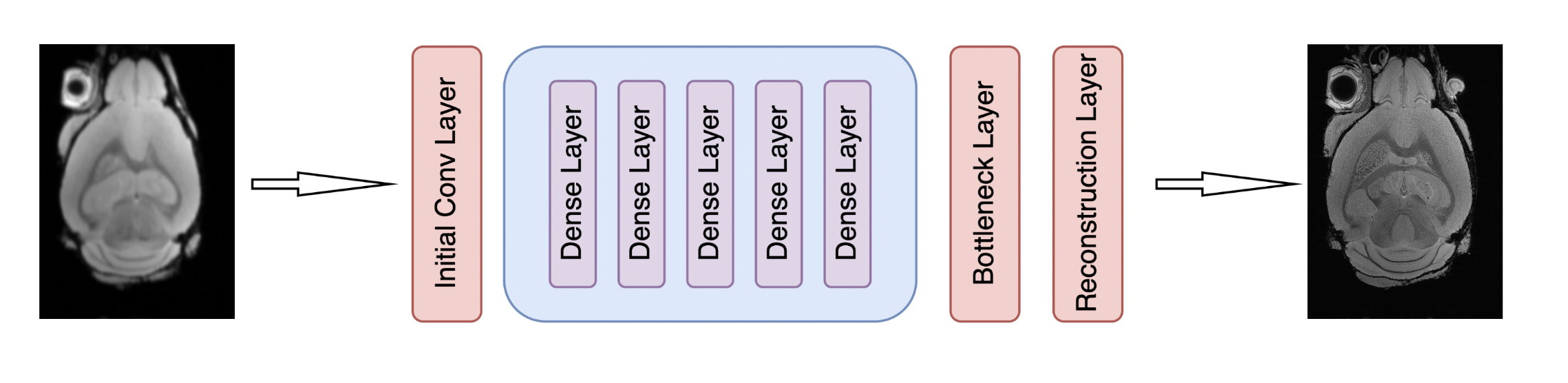
Data set and Training Sample Preparation: All experiments were carried out in compliance with the local Institutional Animal Care and Use Committee. Five Alzheimer’s disease (AD) with 5xFAD background mice brains were acquired on a 30-cm bore 9.4 T magnet (BrukerBioSpec 94/30, Billerica, MA). A 3D gradient echo (GRE) pulse sequence was performed at the spatial resolution of 25 × 25 × 25 μm3, FOV = 18.0 mm × 12.8 mm × 7.6 mm, flip angle = 45°, bandwidth (BW) = 125 kHz, and TR = 100 ms. To investigate the bias of the model, we used these images as High-Resolution images and created 6 different training sets each of size $$$T = 720 $$$ using 6 different degradation models such as Gaussian, Hamming, Hanning, Bicubic, Mean and Median Filtering to mimic low-resolution images and corresponding 6 validation sets. We train a DL framework six different times using these 6 training sets separately and saved all 6 trained DL models. We also created a training set having the same number of training samples $$$T= 720 $$$ but containing an equal proportion of examples from each of the six degradations models to investigate the performance of the DL super-resolution framework when degradation diversity is enforced in training.
Deep Learning Architecture: We used a DenseNet architecture ⁷ as shown in Fig (2) as our DL framework. We used a network with 5 dense blocks each block consisting of 5 convolution layers with a growth rate of 5. Convolution layers have a kernel size 3 with stride and padding equal to 1, for all experiments.

Result and Discussions

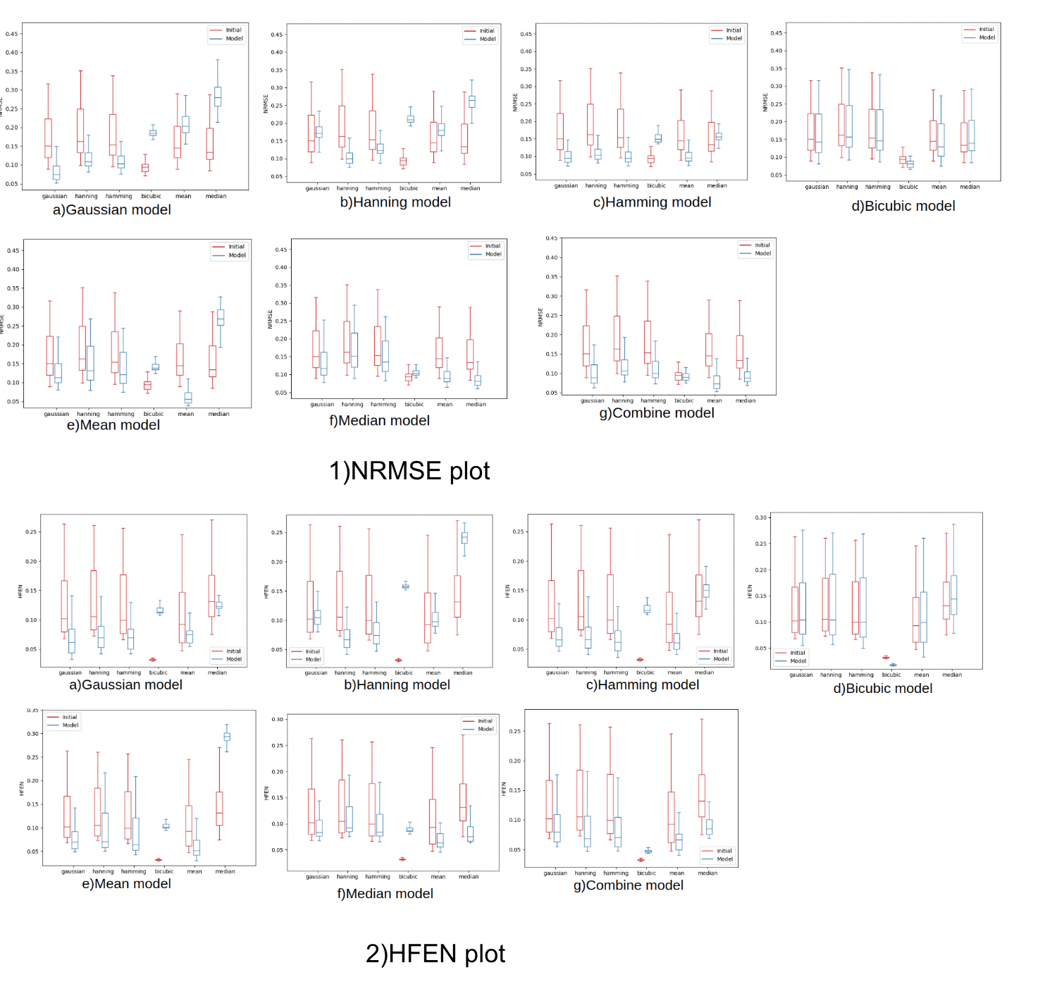
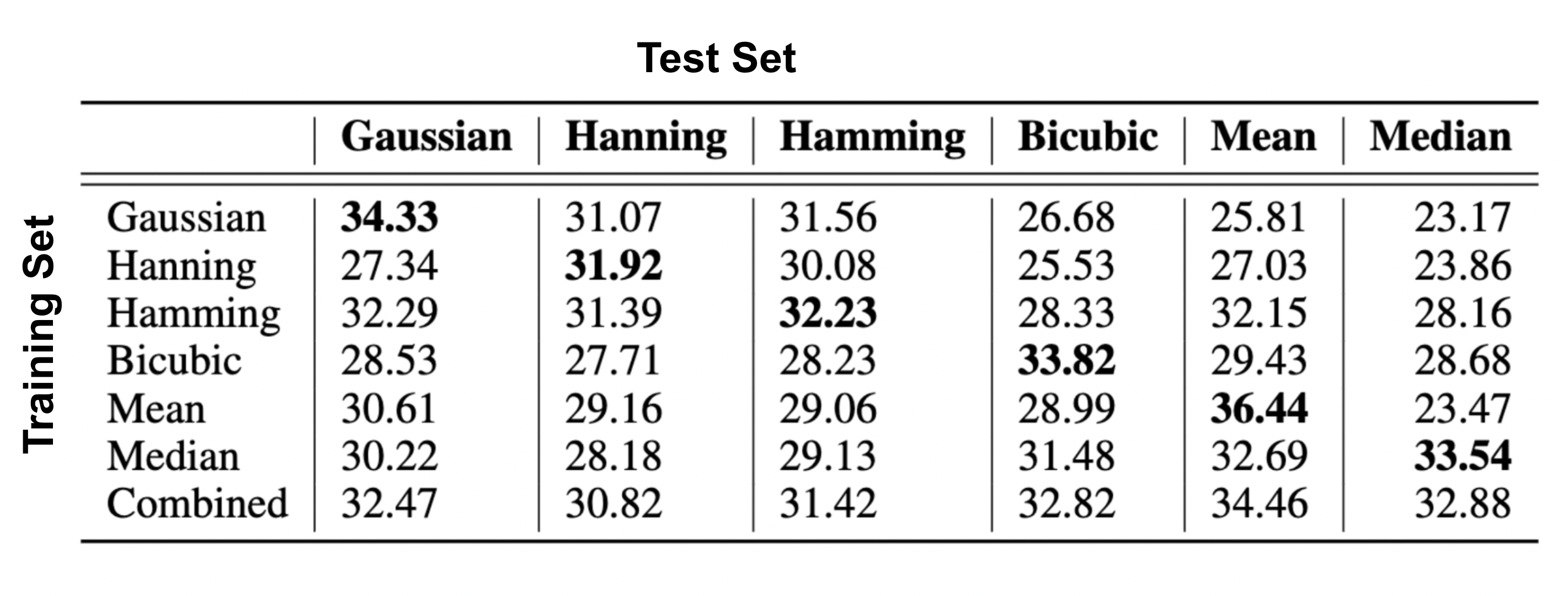
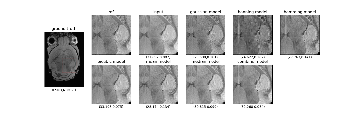
Figure 3 shows NRMSE and HFEN ⁸ performance metrics for 7 different experiments each representing 7 different $$$\phi(\cdot)$$$ used to train the deep learning framework. We can see when model $$$\phi(\cdot)$$$ in the training and validation set is the same, both NRMSE and HFEN have the best metric compared to all other 5 validation sets suggesting that the DL framework is biased on degradation model is used for the training. However, the model trained with training data using all 6 degradation models (combined model), but with the same T, has consistent and robust performance across all validation data. The same conclusion can be derived from Figure 4 which shows the average PSNR for all experiments. Figure 5 shows a representative super-resolution image reflecting the bias of a DL framework trained on bicubic modeling of low-resolution images.

Conclusion

We investigated the bias of deep learning frameworks on training data. We found that the degradation model produces poor results when the degradation of the test set differs from that of the training set. Deep learning super-resolution framework trained and tested on incorrectly modeled low-resolution and high-resolution image pairs can give misleading performance metrics.

Acknowledgements

No acknowledgement found.