Synopsis

Keywords: Image Reconstruction, Machine Learning/Artificial Intelligence

Although recent studies enabled physics-guided deep learning (PG-DL) reconstruction of 3D non-Cartesian MRI, it suffers from blurring, partially due to limited training data. In this study we propose 2.5D PG-DL using three 2D CNNs on orthogonal views for 3D reconstruction to efficiently exploit the limited training data. Results on 3D kooshball coronary MRI show the proposed strategy noticeably improves image sharpness.

Introduction

Recent progress on memory-efficient deep learning techniques^1-3 has enabled physics-guided deep learning (PG-DL) reconstruction^4-6 of large-scale non-Cartesian MRI⁷. Although it tackled hardware limitations, naïve PG-DL of 3D non-Cartesian MRI suffers from blurring at high acceleration rates, hindering its practicality. This is partly due to limited training data, since the whole 3D volume has to be used for training, requiring hundreds of fully-sampled scans to be completed prior to training. In this study, to address this challenge, we employ a 2.5D strategy, which has been previously used in classification-type tasks⁸, for PG-DL reconstruction of 3D kooshball datasets. This 2.5D PG-DL uses three 2D CNNs over coronal, sagittal and axial planes individually. Thus, each 3D training data is treated as a large batch of 2D images to support the training of deep 2D CNNs. Results show that the proposed method visibly improves image quality and sharpness compared to earlier prototype 3D PG-DL reconstruction⁷.

Methods

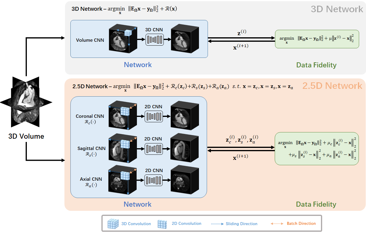
PG-DL Formulation: Regularized MRI reconstruction solves the inverse problem:
$$arg\min_{{\bf x}} ||{\bf Ex - y}||^2_2 + \mathcal{R}({\bf x})$$
where $$$\bf E$$$ denotes the multi-coil encoding operator, $$$\bf x$$$ s the underlying image, $$$\bf y$$$ is the acquired data in k-space, and $$$\mathcal{R}({\cdot})$$$ is a regularizer. In PG-DL, (1) is often solved via algorithm unrolling using a fixed number of iteration steps, where each iteration performs a linear data-fidelity (DF) and CNN-based regularization⁶.
2.5D Network for Limited 3D Training Data: To better utilize the limited training data, we propose a 2.5D approach instead of its 3D counterpart. Three 2D CNN-based regularizers $$$\mathcal{R}_c({\bf x})$$$, $$$\mathcal{R}_s({\bf x})$$$, $$$\mathcal{R}_a({\bf x})$$$ performs 2D convolutions over coronal, sagittal and axial planes respectively. Effectively, each 2D CNN treats 3D training data as a batch of 2D images (Fig. 1). The resulting 2.5D PG-DL reconstruction is formulated as:
$$ arg\min_{{\bf x}} ||{\bf Ex - y}||^2_2 + \mathcal{R}_c({\bf z}_c) + \mathcal{R}_s({\bf z}_s) + \mathcal{R}_a({\bf z}_a) $$
$$ {\it s.t.} {\bf x = {\bf z}_c = {\bf z}_s = {\bf z}_a} $$
which leads to the unconstrained problem:
$$ arg\min_{{\bf x}} ||{\bf Ex - y}||^2_2 + \mathcal{R}_c({\bf z}_c) + \mathcal{R}_s({\bf z}_s) + \mathcal{R}_a({\bf z}_a) + \mu_c||{\bf x} - {\bf z}_c||^2_2+\mu_s||{\bf x} - {\bf z}_s||^2_2+\mu_a||{\bf x} - {\bf z}_a||^2_2$$
he corresponding unrolled steps for solving (3) are:
$$ {\bf z}^{(i)}_c = \mu_c||{\bf x} - {\bf z}_c||^2_2 + \mathcal{R}_c({\bf z}_c) $$
$$ {\bf z}^{(i)}_s = \mu_s||{\bf x} - {\bf z}_s||^2_2 + \mathcal{R}_s({\bf z}_s) $$
$$ {\bf z}^{(i)}_a = \mu_a||{\bf x} - {\bf z}_a||^2_2 + \mathcal{R}_a({\bf z}_a) $$
$$ {\bf x}^{(i+1)} = ({\bf E}^H{\bf E} + (\mu_c + \mu_s + \mu_a){\bf I})^{-1}({\bf E}^H{\bf y} + \mu_c{\bf z}_c+ \mu_s{\bf z}_s+ \mu_a{\bf z}_a)$$
Imaging Data: A research 3D kooshball coronary MRI pulse sequence was acquired using a clinical 1.5T scanner (Magnetom Aera, Siemens Healthcare, Erlangen, Germany) on 8 subjects, using an ECG-triggered T2-prepared, fat-saturated, navigator-gated bSSFP sequence. Relevant imaging parameters: resolution=(1.15mm)³, matrix size=192³, FOV=(220mm)³ with 2-fold readout oversampling. A total of 12320 radial projections (sub-Nyquist rate of 5) were acquired in 385 heartbeats with the spiral phyllotaxis pattern⁹ with one interleaf of 32 readouts per heartbeat. The data was further retrospectively sampled by 6-fold prior to any processing.
Training Details: 2.5D and 3D PG-DL using 10 unrolled steps were implemented as is described in⁷. Training was performed on six subjects, and testing on 2 distinct subjects. Linear DF was solved with a relaxation parameter individually learned for each unrolled iteration, while the CNNs were shared across iterations. 3D PG-DL used ResNet10 regularizer with 3×3×3 convolutions. 2.5D PG-DL used three ResNets of the same architecture with 3×3 convolutions. Under this setup, 3D and 2.5D networks had the same number of learnable parameters (1,444,611).

Results

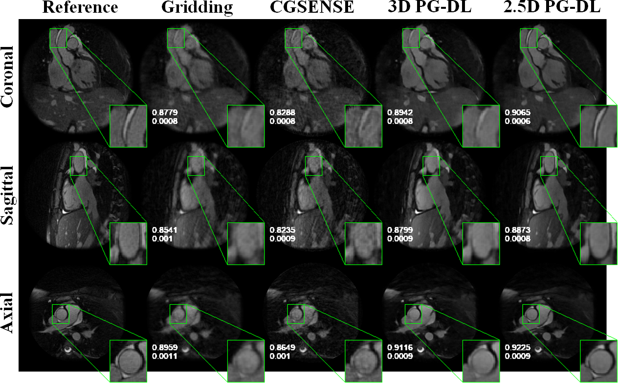
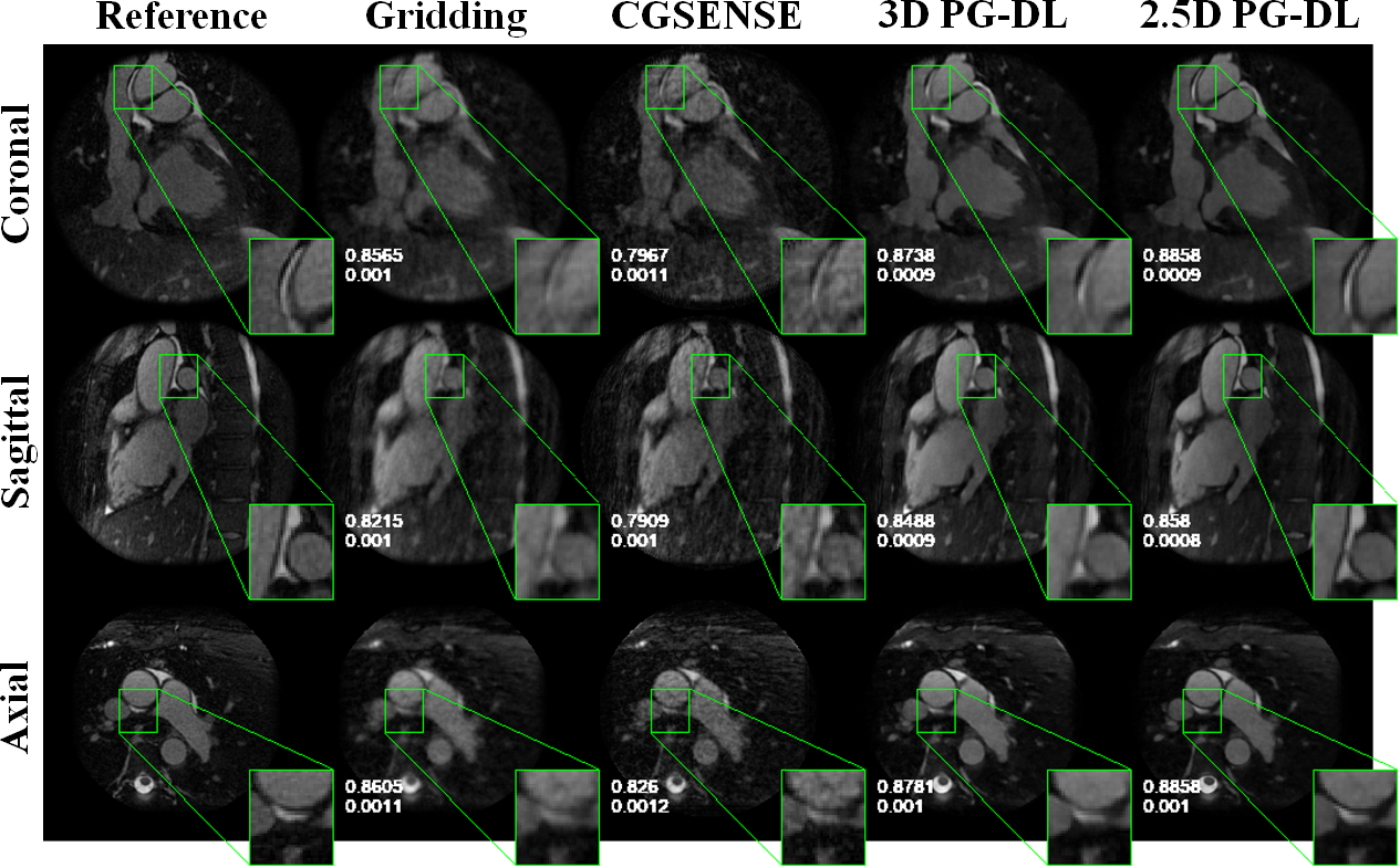
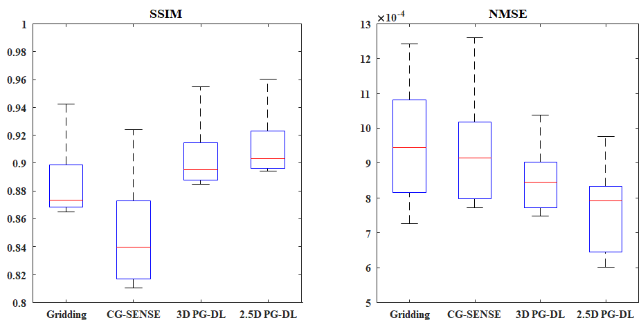
Fig. 2 and 3 depict representative reconstructions from 2 distinct subjects, in coronal, sagittal and axial views, both with 6-fold acceleration. Due to the high acceleration rate, gridding reconstruction shows noticeable artifacts, while CG-SENSE shows noise amplification. Conventional 3D PG-DL⁷ shows better noise suppression albeit visible blurring. The proposed 2.5D PG-DL outperforms the other methods in terms of noise and artifacts, improving image sharpness. SSIM and NMSE of the respective slices reported in the figures align with these visual assessments. Fig. 4 depicts SSIM and NMSE over all 2D slices, showing the median and interquartile ranges. 2.5 PG-DL significantly outperforms all methods (P<0.05).

Discussion and Conclusion

In this study, we improved PG-DL reconstruction of 3D non-Cartesian MRI using 2.5D networks, which efficiently utilized the limited training data. The result shows proposed 2.5D networks offer visible improvement on image sharpness compared to 3D processing.

Acknowledgements

This work was partially supported by NIH R01HL153146, NIH P41EB027061, NIH R21EB028369, NSF CAREER CCF-1651825.