Synopsis

Keywords: Machine Learning/Artificial Intelligence, Quantitative Imaging, SPION

SPION is a contrast agent with a wide range of biomedical applications. A new Deep Learning based method is presented for the quantification of SPION from intensity images. This contrast agent cause off-resonance artifacts, distorting the image. The field map is encoded in the difference of two images taken alternating the direction of the slice selection gradient. The network was trained on simulated data. The network is based on U-net and uses only 2D convolution to process the whole 3D volume, interpreting the last dimension as filters. Results are shown in simulations and on phantoms acquired on a 7T scanner.

Introduction

Quantifying the concentration of SPION density in an MRI image can be a useful biomarker for the presence of sentinel node metastasis¹. SPION are also used as a contrast agent in detecting liver metastases², MR angiography, and tracking in-vivo labeled cells³. Previous methods for estimating the concentration of SPION rely on the image phase. These methods do not work well for large concentrations of SPION because the signal decays rapidly, and the phase becomes unreliable. In 2020, it was demonstrated by della Maggiora⁴ that SPION can be quantified from the magnitude using the View Line sequence. This sequence is long because it requires many images to obtain the excitation profile on a line-by-line basis. In this work, we propose a novel method for generating a concentration map of the SPION from two intensity images.

Methods

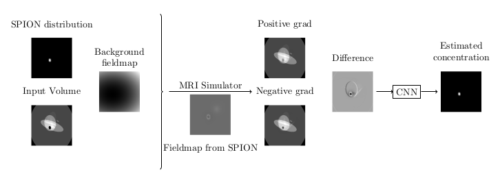
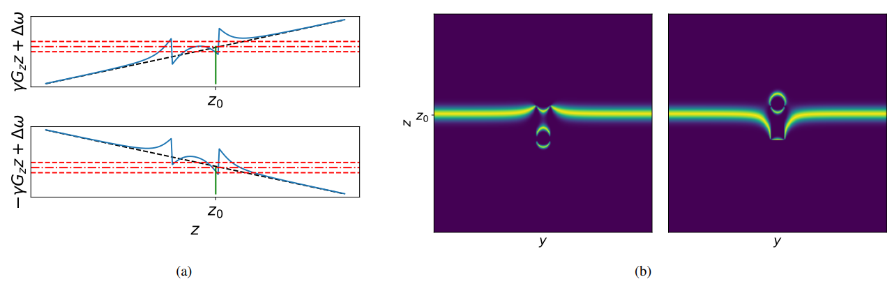
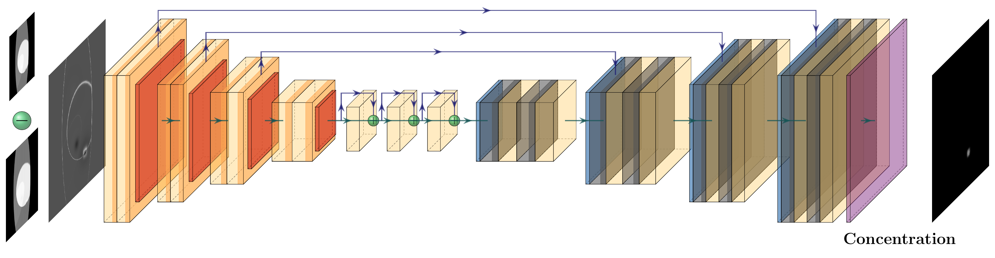
Off-resonance changes the magnitude of the image, but these changes are confused with the magnitude of the object; therefore, there is a need to encode the field map. To do this, we exploit the fact that the artifacts depend on the acquisition parameters. We propose acquiring two images and alternating the direction of the slice selection gradient between them. This will produce images with different artifacts, and the difference will encode information about the field map (see figure 2). We hypothesize that a convolutional neural network (CNN) can learn to extract the SPION concentration from this difference.


The training was done on a simulated dataset of random shapes (similar to DeepQSM⁵). The data was generated using a custom-made simulator tuned to produce realistic images. The input is the difference between the two alternating gradient images, and the output is the concentration map.

The artifacts due to off-resonance are geometric distortions in the through-plane direction. This implies that the data has to be looked at as a volume instead of multiple independent slices. Unfortunately, a full 3D network can be cost-prohibited⁶. We propose to use a 2D network where the third dimension is treated as a different channel of a 2D image, similar to ref⁷. The 3D relationship is not lost because the convolution operator is summed over the channels to form the output activation, effectively doing a weighted sum across the third dimension. We oriented the sample so that the filter axis is in-plane, and the convolutions were performed in the plane containing the selection direction, where the off-resonance effects are more noticeable.

The loss function has two terms: the normalized mean square error (NMSE) to focus on the SPION concentration estimation and the DICE loss to focus on the shape of the prediction. We also regularize the network output to promote sparsity using an l1-norm. All the code for data generation and training is available at https://gitlab.com/asdibiase/spion-estimation.

Results

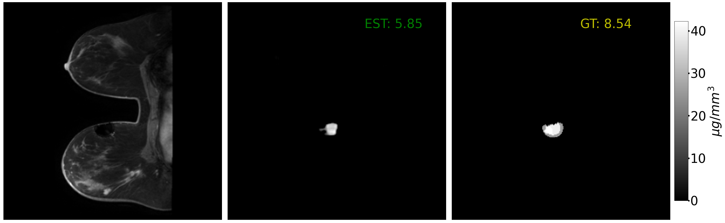
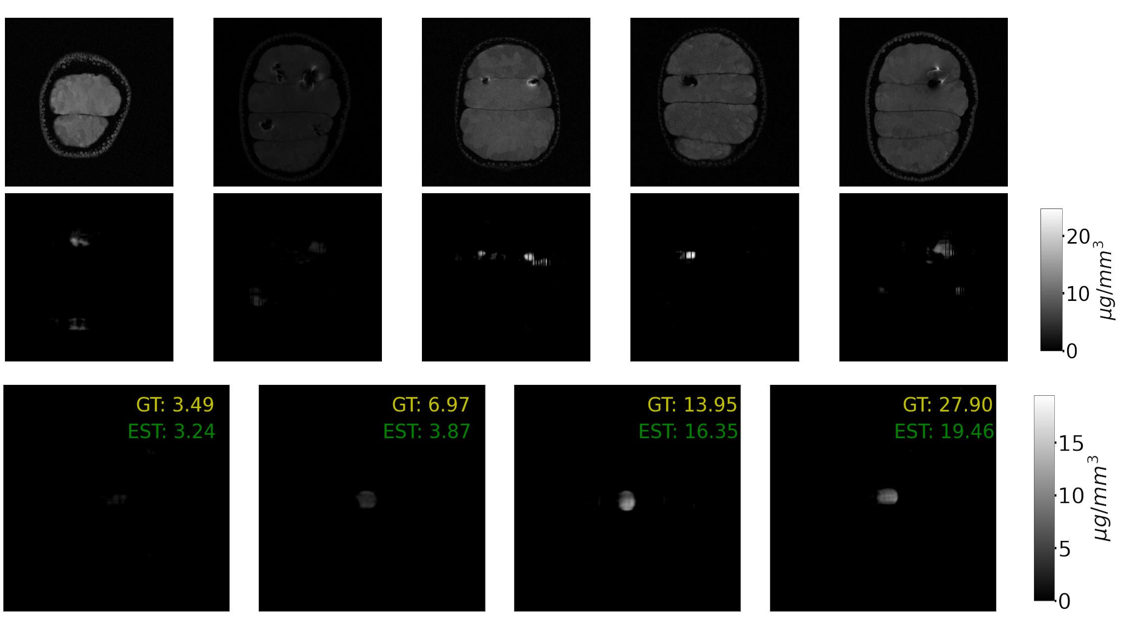
To evaluate the performance of the proposed method; we run experiments on simulations and data from a 7T scanner. To ensure our method does not present any bias towards the synthetic shapes used during training, we simulated adding a blob of SPION to a breast MRI from the RIDER dataset^8,9. The image can be seen in figure 4 with an NMSE of 0.7355. We found that there is no bias because the concentration is accurately predicted. We attribute this to the fact that the input to the network is the difference of alternating gradient images, effectively eliminating everything but the SPION artifacts.

Next, we tested the method on images acquired at a 7T scanner. We tested the accuracy of the predictions using cylindrical vials with different concentrations of SPION. The results can be seen in figure 5 (bottom). Then we imaged oranges injected with SPION. The results are shown in figure 5 (top). We can see that each dark spot in the original image (top row) corresponds with a blob of predicted SPION in the bottom row.

Discusssion and conclusions

We propose a new method for estimating the concentration of SPION with a CNN from two magnitude-only MR images. The training was done using simulated images. This method can estimate the concentration in all tested examples (simulated and acquired data). In contrast to previous methods, ours only needs a pair of intensity images, greatly reducing imaging time and not requiring any special sequence.

Although the estimation of the maximum concentration has errors of up to 45%, the general shape of the distribution is well predicted and in the range of the expected accuracy. Despite this relatively low accuracy, our method can estimate the concentration in regions with no signal and where all methods based on the phase would fail.

Some results of the predicted concentration present black vertical lines (see figure 5). The network sees this dimension as a filter and can only be filled with a linear combination of previous features, which may not contain enough information to build a continuous image. A possible solution to this problem is to increase the number of filters in the network to allow for a more expressive representation.

Acknowledgements

A. D. and P. I. acknowledge support from ANID grant FONDECYT 1210747 and from ANID, Millennium Institute for Intelligent Healthcare Engineering (iHEALTH) ICN2021 004.