Synopsis

Keywords: Sparse & Low-Rank Models, Arterial spin labelling

ASLfMRI temporal SNR (tSNR) and sharpness in the inferior-superior direction was improved by using partial separability, a low rank model. The method requires an additional novelty to the partial separable model which allows time points with no corresponding imaging data, only temporal navigator data, to be reconstructed. A finger tapping task was used to demonstrate the detection of cerebral blood flow to the motor cortex. Mean squared error, structural similarity index, and the area under the curve of a receiver operating characteristic curve was also improved as shown by using a simulation of ASLfMRI data.

Introduction

ASLfMRI can be a valuable tool to assess brain function¹. Partial separability is a method that has been used to reconstruct subsampled MRI data by exploiting low-rank spatiotemporal correlations^2,3,4,5. The partial separability model can also be applied to ASL functional imaging, evidenced by previous work using a low-rank method with Robust Principal Components Analysis for ASLfMRI⁶. However, model based ASL reconstructions model the perfusion signal and therefore require subtractions of the control/label pairs before reconstruction. This pre-reconstruction subtraction has been used previously in a model-based method using dictionary learning⁷. Because the partial separable model requires that control and label images in the same pair have the same sampling scheme (shot of k-space), subtracting the images before reconstruction decreases the temporal resolution by a factor of 2. Here a reconstruction called PSASLfMRI (PS) is implemented which uses navigator data to reconstruct control/label pairs that have a different sampling scheme. Therefore, a running subtraction could be used to preserve temporal resolution⁸. Simulations using a numerical phantom were run to test the method to obtain specificity and sensitivity estimates and human data was used to verify the method with a finger tapping task.

Methods

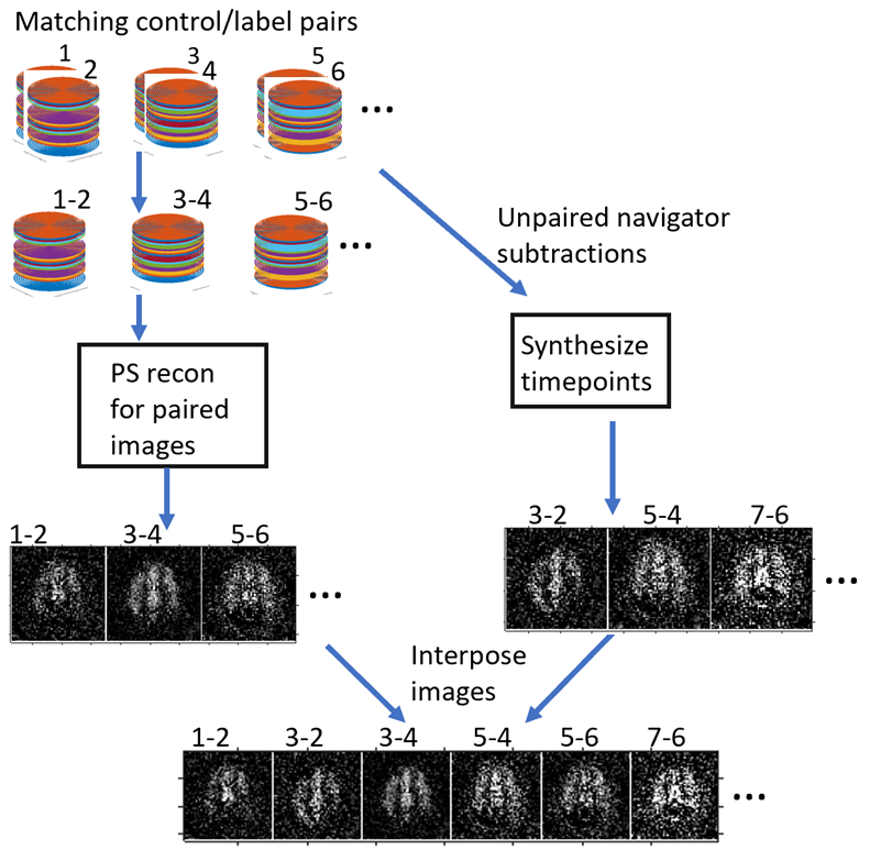
In-plane spirals were used with 3D FAIR PASL. The nonuniform fast Fourier transform algorithm was used to accommodate the non-uniform sampling⁹. The image dimensions were 64x64x32, 162 repetitions were acquired, and the TR was 4 seconds. Other protocols followed the ASL consensus paper¹⁰. Data were collected and reconstructed in two ways: 1. Fully sampled data to allow a running magnitude subtraction with a standard reconstruction, with partial background suppression. 2. 16/32 kz-line undersampled data with a navigator of 5 center spirals in kz, with PS reconstruction with full background suppression followed by synthesizing the subtracted control/label pairs which had no matching imaging data besides the navigator. The PS model was used as described previously²: $$c_l(k)=arg\min_{c_l(k)}||s(k,t)-\sum_{l=1}^Lc_l(k)\rho_l(t)||^2$$ where $$$L$$$ is the rank of the reconstruction, which was set to 27 based on examining the temporal basis for relevant ASL signal. $$$t$$$ is the time point, $$$c_l(k)$$$ is the estimated spatial basis, $$$s(k,t)$$$ is the acquired data, and $$$\rho_l(t)$$$ is the estimated temporal basis. 15 iterations of conjugate gradient were used for each reconstruction.
To solve for the subtracted control/label pairs that did not have matching imaging data, the following algorithm was implemented: $$v_l(t)=s_l^{-1}u_l^*(k)n(t)$$ Where $$$v_l(t)$$$ are the temporal basis functions corresponding to subtractions without matching imaging data and $$$n(t)$$$ is the subtracted navigator corresponding to subtractions without matching imaging data. $$$u_l(k)$$$ and $$$s_l(t)$$$ are the left singular vector matrix and the corresponding singular value of the original navigator, respectively (* is complex conjugate). The two temporal basis functions were interposed to create a temporal basis for the entire time series. The new temporal basis and the spatial basis $$$c_l(k)$$$ were multiplied and the real part was taken as the PS reconstruction (Figure 1).
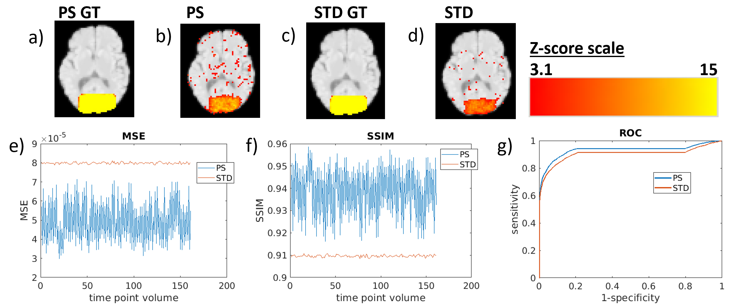
A human brain MPRAGE was segmented to create the numerical phantom with gray matter, white matter, CSF, and blood with the proper proton densities, perfusion, and T2 weighting. Background suppression was calculated for each tissue and the blood¹¹. Stimulation was simulated to be a 90% increase in blood signal in a 20 seconds off 20 seconds on pattern. A 3D gaussian kernel 5x5x5 pixels, with a small standard deviation for each time point for randomness, was convolved with the phantom. The phantoms were then sent through the PS and STD reconstructions. Gaussian noise was added to the real and imaginary parts of the k-space data. Running subtractions of the numerical phantoms were passed into the fMRI software and their activations maps were used as ground truth. The activations were calculated using FSL FEAT¹² with cluster corrected threshold, and the resulting Z-score statistics were used to create the ROC curve in Figure 2.
A 3T MRI scanner was used for real-world data collection. Voxel sizes were 3.8x3.8x3mm. A task that consisted of 20 seconds of rest and 20 seconds of finger tapping increased blood flow to the motor cortex. The data was sent through FSL FEAT with the same settings as the simulation with a higher Z-score threshold used for PS to control spurious activation from the PS method.

Results

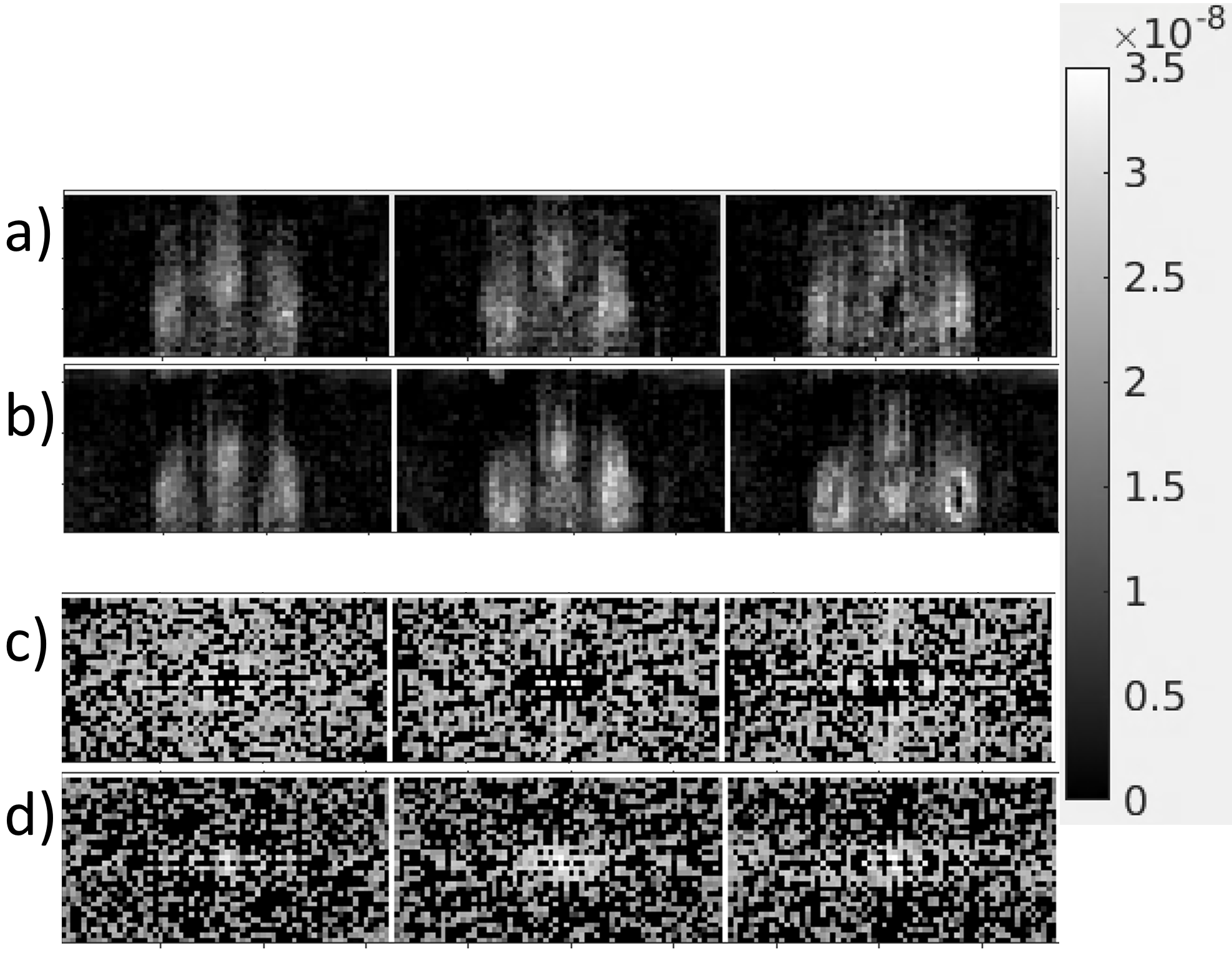
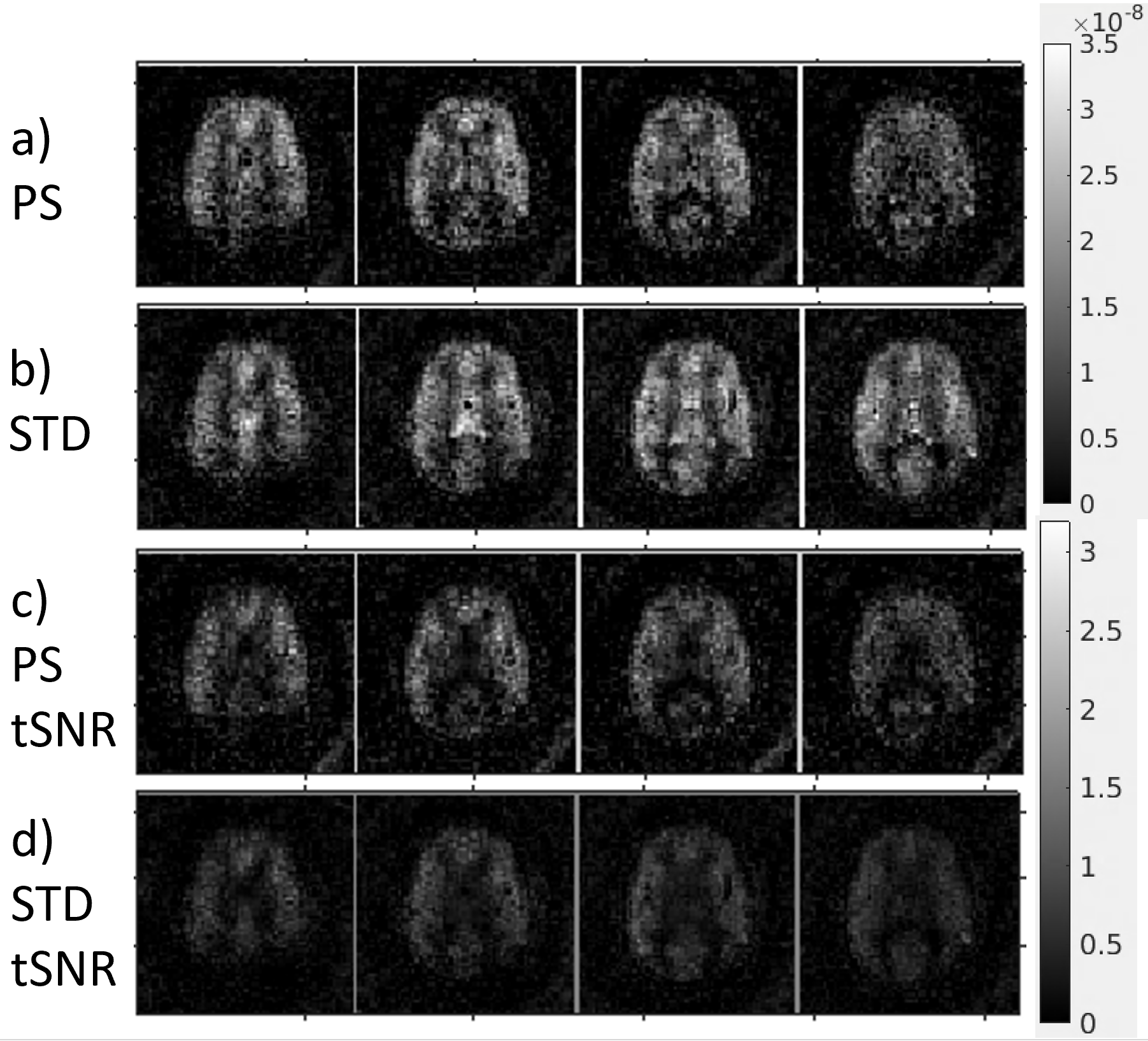
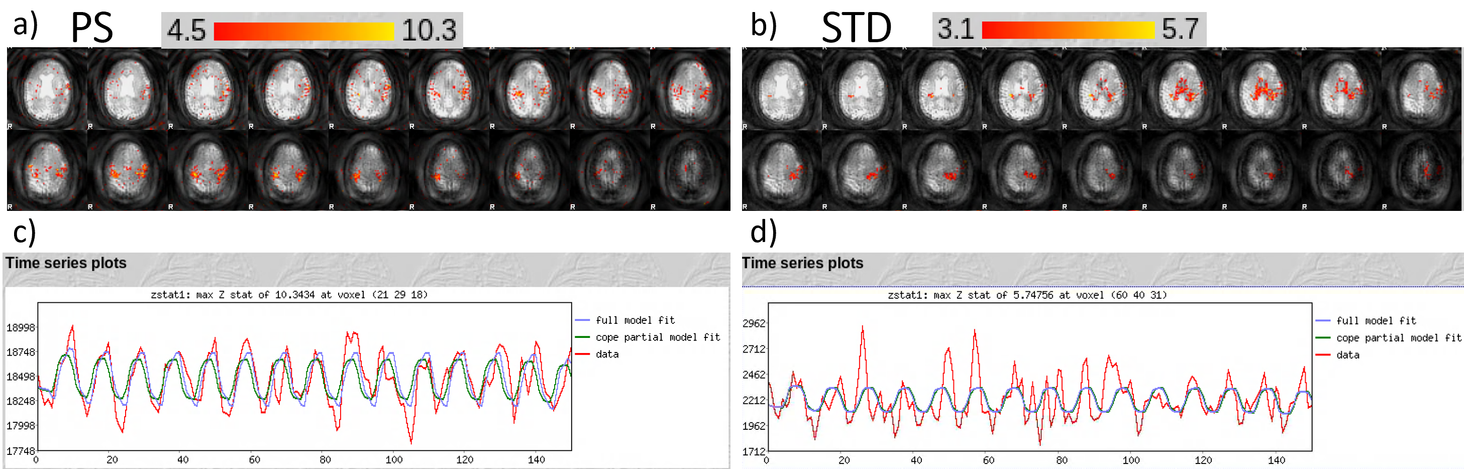
Figure 2 shows that the PS has a lower MSE, a higher SSIM, and a higher AUC compared to STD using the simulation. Figure 3 shows that PS has a higher sharpness in the coronal direction due to higher signal in the higher spatial frequencies. Figure 4 shows that PS has a higher tSNR than STD. Figure 5 shows the activation maps for PS detects activation of the motor cortex due to finger tapping.

Discussion

The simulation shows the PS method allows for a more accurate reconstruction and a more sensitive and specific measure of brain function at least for the simple simulation. The sharper result for the human data can be obtained using the PS method, which is due to less T2 decay that happens because of subsampling k-space. The reduction in the rank also increases the tSNR. The results of the finger tapping task show that the PS reconstruction captures blood flow activation.

Acknowledgements

This work was supported by the Miniature Brain Machinery Fellowship, training grant number NSF 1735252.