2872
Consideration of peripheral nerve stimulation in the optimization of spiral k-space trajectories
Oliver Schad1,2, Tobias Wech1, and Herbert Köstler1
1Department of Diagnostic and Interventional Radiology, University Hospital Würzburg, Würzburg, Germany, 2University of Würzburg, Experimental Physics 5, Würzburg, Germany
1Department of Diagnostic and Interventional Radiology, University Hospital Würzburg, Würzburg, Germany, 2University of Würzburg, Experimental Physics 5, Würzburg, Germany
Synopsis
Keywords: Gradients, Safety, Peripheral Nerve Stimulation
The algorithm we present in this work designs variable density spiral (VDS) trajectories and their respective gradient time courses based on the Stanford VDS-tool. In addition to hardware limits (maximum gradient strength and slew rate) a PNS threshold based on the SAFE-Model is introduced.Purpose
To consider peripheral nerve stimulation restrictions for the automatic design of spiral k-space trajectories.Introduction
Peripheral nerve stimulation (PNS) can occur in MR imaging of patients due to time varying magnetic fields. The scanner manufacturers therefore implement security routines that prohibit the execution of critical gradient waveforms, in compliance with the regulating standard.For common gradient systems and manifold applications, the optimization of spiral trajectories is frequently limited by PNS and not only by maximum gradient strength and slew rate.
Schulte et al. 1 proposed the design of PNS optimized spirals using a convolution model, showing increased scan efficiency in comparison to spirals with globally reduced slew rate. Unfortunately, scanner manufacturers use different models to predict PNS. On Siemens scanners the so-called SAFE-model (Stimulation Approximation by Filtering and Evaluation 2) is implemented. In this work, we present the design of PNS optimized spiral trajectories using the SAFE-model in order to generate time efficient gradient courses on a Siemens MAGNETOM Avanto system.
Methods
Providing arbitrary gradient time courses $$$G_i(t)$$$ on the respective physical scanner axis (i=x,y,z), the SAFE-model calculates the resulting nerve response $$$R_i(t)$$$ using various coil-specific lowpass-filters, rectifiers and scaling factors for the individual axis. A schematic illustration of the calculation process is shown in Fig. 1. After differentiation of $$$G_i(t)$$$ the time course is split into three branches, each applying a RC-lowpass filter with time constant $$$\tau$$$, taking the absolute value and scaling with a factor $$$a$$$. In the second branch, filtering and taking the absolute value are permuted. The sum of the three contributions is then again scaled with an axis specific factor $$$g_i$$$ leading to the nerve response of the respective axis. The overall stimulation time course is then given by $$$PNS_\text{tot}=100\,\sqrt{R_x^2+R_y^2+R_z^2}$$$. Since the y-coil induces the strongest stimulation impulse, the physical axis are unified by only considering the parameters of the y-axis for our calculations.The main algorithm is created based on the VDS Matlab tool by Brian Hargreaves 3. Here, the spiral trajectories start in a slew rate ($$$SR_\text{max}$$$) limited regime until the maximum gradient strength ($$$G_\text{max}$$$) is reached, which is then kept constant. Each point of the trajectory is calculated iteratively by solving a quadratic equation, resulting from the analytical description of the trajectory and using the solution with positive sign to traverse the trajectory. While the positive solution increases the gradient strength and stimulation, the negative solution generally leads to a decrease.
We introduced a PNS-limited domain, by simultaneously calculating the PNS time course for each step of the trajectory and considering positive and negative solutions for the next time step. If the positive solution of the quadratic equation leads to a stimulation threshold overshoot, while the negative solution does not, a linear interpolation between the two solutions is performed. Assuming that the stimulation model can be linearly approximated for short time intervals, PNS can be kept constant by this approach.
A schematic illustration of this process is shown in Fig. 2. In order to follow a given trajectory path, the gradients must be adjusted using the available slew rate. The green circle depicts all possible solutions for the i+2-th k-space point using $$$SR_\text{max}$$$. Its cross-section with the trajectory leads to the two possible solutions (decreasing and increasing gradient strength with $$$SR_\text{max}$$$ respectively). The minimal slew rate $$$SR_\text{min}$$$, required to stay on the trajectory, corresponds to a vanishing root in the solution of the quadratic equation. $$$SR_\text{min}$$$ keeps the gradient strength constant. By interpolating between the two solutions with $$$SR_\text{max}$$$, another solution can be found, which adjusts the slew rate according to the present PNS restrictions.
Data
An exemplary spiral trajectory was created with the following parameters: $$$SR_\text{max}$$$= 170T/m/s, $$$G_\text{max}$$$= 40mT/m (Avanto gradient coil limits), $$$FOV$$$ = 45cm (decreasing linearly to 15cm at $$$k_\text{max}$$$), $$$res$$$ = 1.5mm x 1.5mm, $$$N$$$ = 10 (interleaves). The PNS threshold was set to 100%.Results
The resulting gradient time courses with the respective slew rates and PNS-courses are shown in Fig. 3. The original algorithm leads to a maximum stimulation of 116% and a duration of 8.46ms. Since $$$G_\text{max}$$$ is not reached, the gradient strength increases steadily with $$$SR_\text{max}$$$. The optimized method keeps PNS constant, decreasing the gradient strength and the slew rate only when necessary, and even increasing it, when possible. The duration of the PNS-optimized trajectory increased by 1.7% to 8.60ms.Discussion
We propose an altered version of the Stanford VDS algorithm, which now also considers solutions with decreasing gradient strength for the purpose of complying with PNS restrictions.The proposed strategy enables a versatile optimization of spiral trajectories with the potential of applying arbitrary PNS models. For our specific case, the design of time-efficient spiral trajectories for Siemens systems was enabled.
Acknowledgements
We thank Brian Hargreaves for providing the Matlab implementation for the design of variable density spirals (http://mrsrl.stanford.edu/~brian/mritools.html (accessed: 17.06.2022)).We further thank Filip Szczepankiewicz for providing a Matlab implementation of the SAFE-model for the PNS-calculation (https://github.com/filip-szczepankiewicz/safe_pns_prediction).
References
1. Schulte, R.F. and Noeske, R. (2015), Peripheral nerve stimulation-optimal gradient waveform design. Magn. Reson. Med., 74: 518-522. https://doi.org/10.1002/mrm.25440
2. Hebrank F., Gebhardt M. (2000), Safe-Model - A New Method for Predicting Peripheral Nerve Stimulations in MRI, Proc. Intl. Soc. Mag. Reson. Med., 8, Denver, CO, USA. 2007
3. Hargreaves B. (2001), Spin-manipulation methods for efficient magnetic resonance imaging, PhD thesis, Stanford, http://mrsrl.stanford.edu/~brian/mritools.html (accessed: 17.06.2022)
Figures
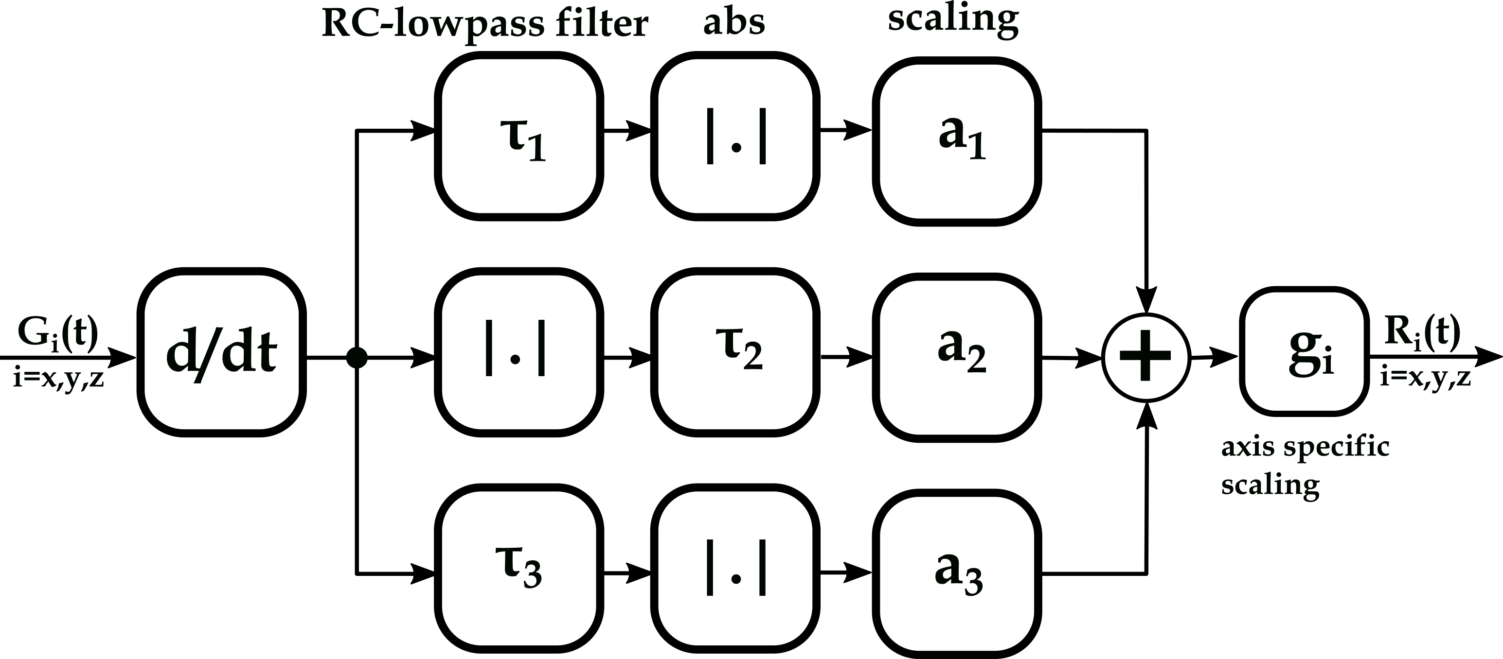
Schematic
illustration of the PNS-calculation using the SAFE-model. After differentiation
of $$$G_i(t)$$$ the time course is split into three branches,
each applying a RC-lowpass filter with time constant $$$\tau$$$,
taking the absolute value and scaling with a factor $$$a$$$. The sum of the three
contributions is then again scaled with an axis specific factor $$$g_i$$$,
leading to the nerve response time course of the respective axis $$$R_i(t)$$$. (adapted
from 2)
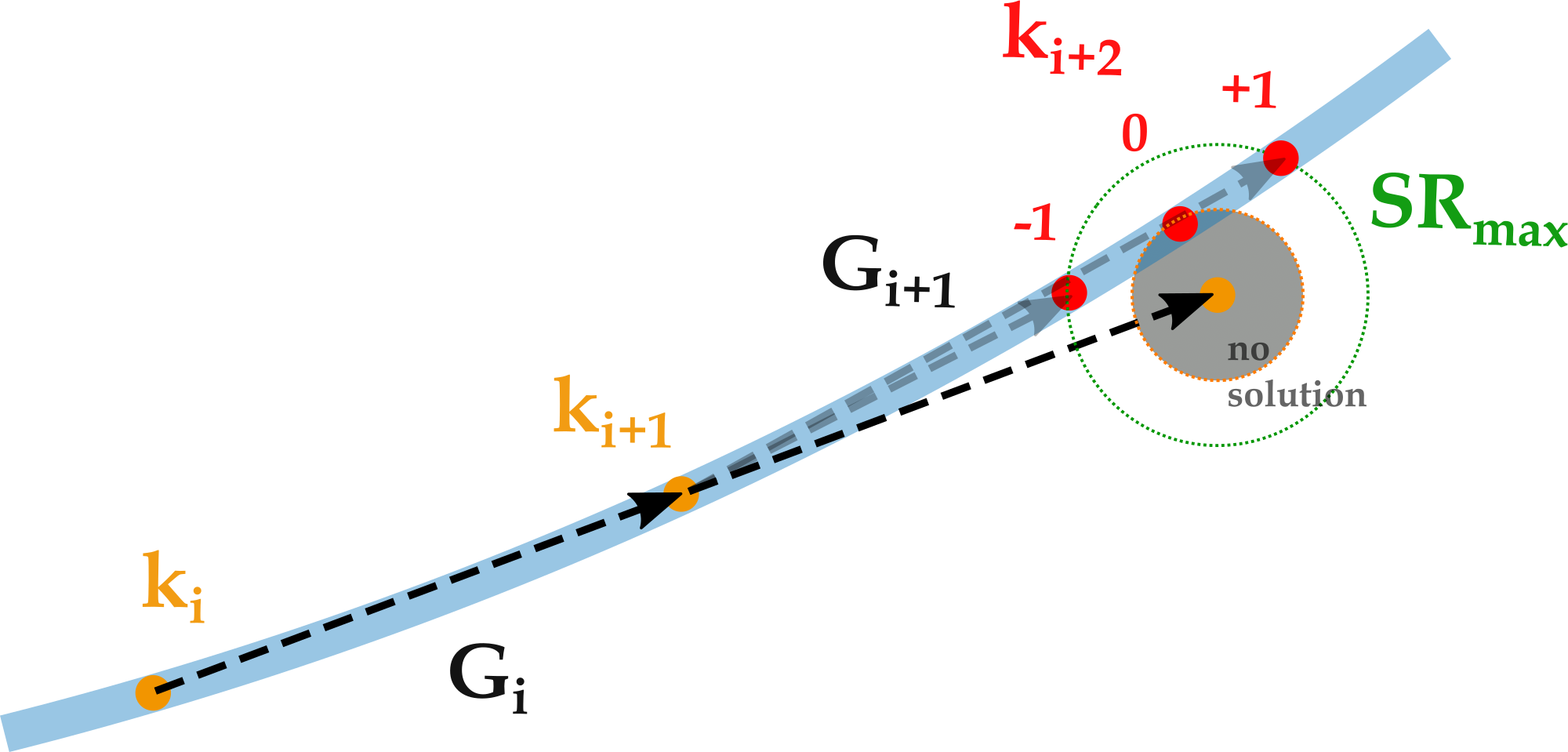
In order to follow a given trajectory, the gradients must be adjusted
using the available slew rate. The green circle depicts all possible positions
for the i+2-th k-space point using $$$SR_\text{max}$$$. Its cross-section with
the trajectory leads to the two possible solutions (decreasing and increasing
gradient strength with $$$SR_\text{max}$$$ respectively). The solution with minimal slew
rate keeps the gradient strength constant, corresponding to a circle touching
the trajectory.
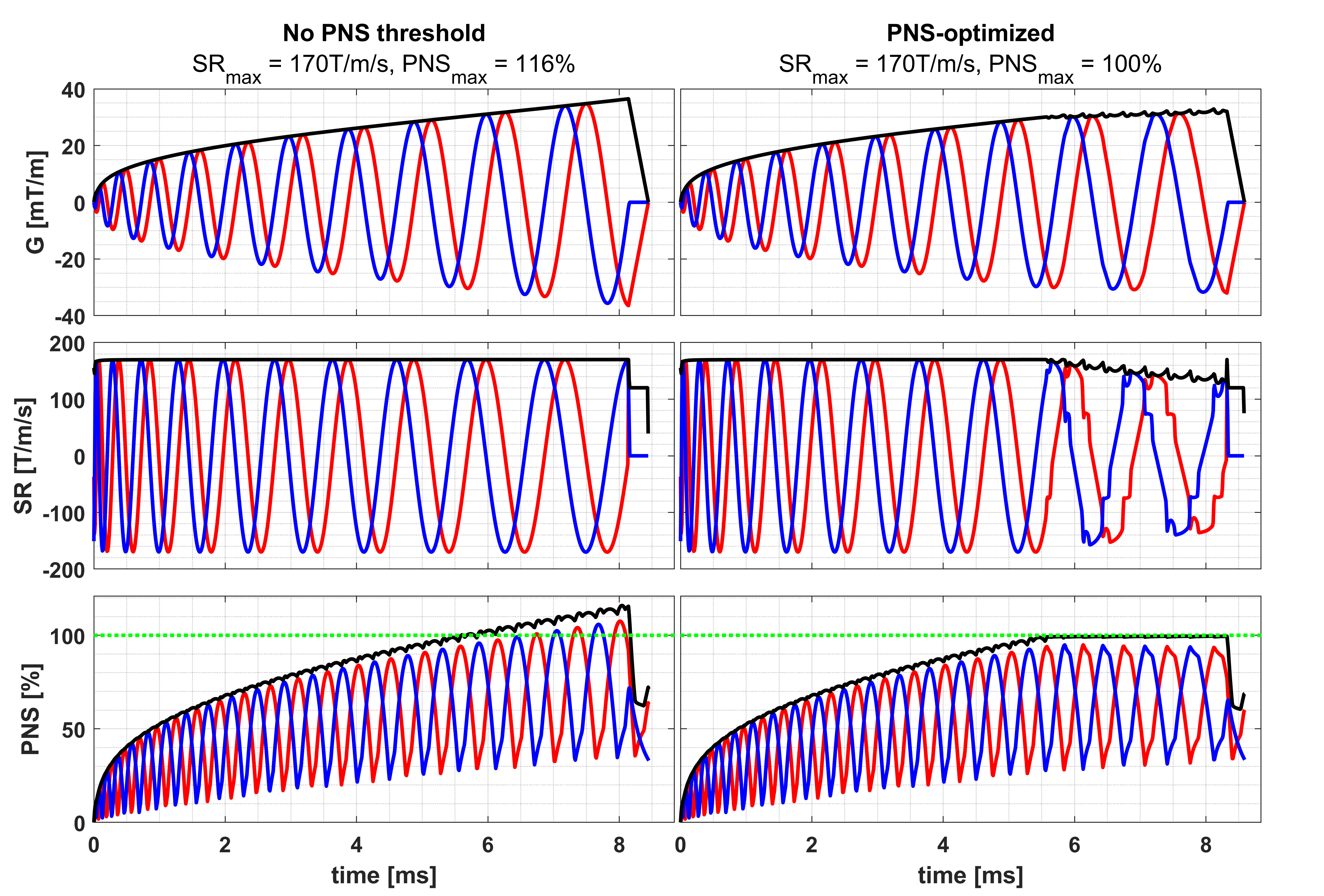
Gradient
(top), slew rate (middle) and PNS (bottom) time courses for an exemplary spiral
trajectory. In the optimized design the slew rate is reduced in order to comply
with the set PNS threshold of 100%, leading to a 1.7% increase in duration in
comparison to the original algorithm.
Blue: x-axis, Red: y-axis, black: respective root sum of squares
DOI: https://doi.org/10.58530/2023/2872