Synopsis

Keywords: White Matter, Relaxometry, Brain, Myelin Water Fraction

$$$T_2$$$ distributions are typically computed using point estimates such as nonnegative least-squares (NNLS). This characterizes the most likely $$$T_2$$$-distribution arising from the data, but disregards other plausible solutions - of which there are many, due to the ill-posed nature of the inverse problem. Here, we instead propose to use Bayesian posterior sampling methods. To guide the difficult high-dimensional sampling problem, a data-driven domain transformation is learned alongside a deep generative prior. The resulting posterior samples produce more spatially consistent myelin water fraction (MWF) maps compared to NNLS, despite the purely voxelwise analysis, and additionally yields novel MWF uncertainty estimates.

Introduction

The $$$T_2$$$-distribution of a multi spin-echo (MSE) magnitude signal is the set of coefficients resulting from a multiexponential signal decomposition. Basis signals are computed using the extended phase graph (EPG) algorithm, incorporating stimulated-echo and $$$B_1$$$-inhomogeneity effects^1,2.
$$$T_2$$$ distributions give insight into tissue microstructure. The myelin water fraction (MWF) of a white matter voxel characterizes myelin content, computed as the relative amount of signal contained in the fast decaying $$$T_2$$$ components^3,4. In luminal water imaging of the prostate, reductions in slowly decaying $$$T_2$$$ components can inform prostate cancer diagnosis^5,6.
$$$T_2$$$ distributions are commonly computed using point estimates such as nonnegative least-squares (NNLS). However, this ignores the large family of $$$T_2$$$ distributions which fit the data nearly equally well due to the ill-posed nature of the problem. Here we use Bayesian posterior sampling methods to quantify the full posterior space of $$$T_2$$$ distributions. Posterior sampling is difficult in high dimensions; to enable efficient sampling, we learn three deep networks: a data-dependent preconditioning transformation of the sampling space, a data-independent deep generative prior to guide sampling, and an encoder to embed the input data into a lower-dimensional representation. Once trained, posterior sampling using Markov chain Monte Carlo (MCMC) is performed in the usual way. This both improves $$$T_2$$$-distribution estimation, and allows us to compute novel uncertainty estimates of the derived MWF.

Methods

Let $$$\mathbf{b}\in\mathbb{R}_+^{n_{\mathrm{TE}}}$$$ be a measured MSE signal, $$$\mathbf{A}\in\mathbb{R}_+^{n_{\mathrm{TE}}\times{}n_{T_2}}$$$ be a matrix of EPG basis signals, and $$$\mathbf{x}\in\mathbb{R}_+^{n_{T_2}}$$$ be a $$$T_2$$$-distribution. The NNLS-based maximum a posteriori probability estimate $$$\mathbf{x}^{*}_{\mu}$$$ is $$\mathbf{x}^{*}_{\mu}=\underset{\mathbf{x}\ge{}0}{\operatorname{arg\,min}}\;||\mathbf{A}\mathbf{x}-\mathbf{b}||_2^2+\mu^2||\mathbf{x}||_2^2.$$ Implicitly, this imposes a uniform Gaussian noise model on $$$\mathbf{b}$$$, with $$$\ell^2$$$-regularization equivalent to a uniform half-normal prior on $$$\mathbf{x}$$$ with scale $$$1/\mu$$$. DECAES⁷ is used to compute $$$\mathbf{x}^{*}_{\mu}$$$, with $$$\mu$$$ determined using the L-curve method^8,9.
Here, we use posterior sampling to capture the diversity of plausible $$$T_2$$$ distributions. Posterior samples $$$\mathbf{x}$$$ are drawn using MCMC with frequency proportional to their posterior probability $$\mathbf{x}\sim{}p(\mathbf{x}|\mathbf{y})\propto{}p(\mathbf{y}|\mathbf{x})p(\mathbf{x})$$ where $$$\mathbf{y}=(\mathbf{A},\mathbf{b})$$$ is the data, $$$p(\mathbf{x})$$$ is the prior distribution over $$$\mathbf{x}$$$, and $$$p(\mathbf{y}|\mathbf{x})$$$ is the likelihood of $$$\mathbf{b}\sim{}\operatorname{Rice}(\mathbf{v}=\mathbf{A}\mathbf{x},\sigma\operatorname{\mathbf{I}})$$$ under Rician noise^10,11 $$\log{}p(\mathbf{y}|\mathbf{x})=\sum_{i=1}^{n_{\mathrm{TE}}}\log\tfrac{\mathbf{b}_{i}}{\sigma^2}+\log\operatorname{I}_0(\tfrac{\mathbf{b}_{i}\mathbf{v}_{i}}{\sigma^2})-\tfrac{\mathbf{b}_{i}^2+\mathbf{v}_{i}^2}{2\sigma^2}.$$ $$$\operatorname{I}_0$$$ is the modified Bessel function of the first kind with order zero. The full posterior includes the noise level $$$\sigma$$$, omitted throughout for brevity: $$$p(\mathbf{x},\sigma|\mathbf{y})\propto{}p(\mathbf{y}|\mathbf{x},\sigma)p(\mathbf{x})p(\sigma)$$$ with $$$p(\sigma)$$$ log-normal corresponding to $$$\text{SNR}=50\pm{}25$$$. Given posterior samples $$$\{\mathbf{x}_{i}\sim{}p(\mathbf{x}|\mathbf{y})\}$$$, statistics of derived metrics $$$\{f(\mathbf{x}_{i})\}$$$ such as MWF are computed as expectations $$$\mathbb{E}_{p(\mathbf{x}|\mathbf{y})} [f(\mathbf{x})] \approx \frac{1}{N} \sum_{i} f(\mathbf{x}_{i})$$$, and similarly for variances, quantiles, etc.
The high-dimensional ($$$n_{T_2}=40$$$) sampling problem is preconditioned through a judicious transformation of the sampling space. Let $$$\mathbf{x}=\varphi(\mathbf{u};\mathbf{y})$$$ be a data-dependent function of an unconstrained vector $$$\mathbf{u}$$$ defining a conditional normalizing flow^12,13 from a base distribution $$$\pi(\mathbf{u})=\mathcal{N}(\operatorname{\mathbf{0}},\operatorname{\mathbf{I}})$$$ onto an approximate posterior $$$q_{\varphi}(\mathbf{x}|\mathbf{y})$$$¹⁴: $$\log{}q_{\varphi}(\mathbf{x}|\mathbf{y})=\log\pi(\mathbf{u})-\sum_{i=1}^{L}\log|\operatorname{det}{\mathbf{J}_{\varphi_{i}}}|$$ where $$$\varphi=\varphi_{L}\circ\cdots\circ\varphi_{1}$$$ is a composition of $$$L$$$ diffeomorphisms $$$\{\varphi_{i}\}_{i=1}^{L}$$$, $$$\mathbf{u}_{i}=\varphi_{i}(\mathbf{u}_{i-1};\mathbf{y})$$$ is the $$$i^{th}$$$ layer output, $$$\mathbf{J}_{\varphi_{i}}=\frac{\partial\mathbf{u}_{i}}{\partial\mathbf{u}_{i-1}}$$$ is the $$$i^{th}$$$ layer Jacobian, and $$$\varphi_{i}$$$ have closed-form Jacobian determinants $$$|\operatorname{det}{\mathbf{J}_{\varphi}}|=\prod_{i=1}^{L}|\operatorname{det}{\mathbf{J}_{\varphi_{i}}}|$$$. Preconditioning via $$$\varphi$$$ transforms the posterior sampling problem into $$\mathbf{u}\sim{}p(\mathbf{u}|\mathbf{y})=p(\mathbf{x}|\mathbf{y})|\operatorname{det}{\mathbf{J}_{\varphi}}|\propto{}p(\mathbf{y}|\mathbf{x})p(\mathbf{x})|\operatorname{det}{\mathbf{J}_{\varphi}}|.$$ If $$$\varphi$$$ is well trained, $$$q_{\varphi}(\mathbf{x}|\mathbf{y})\approx{}p(\mathbf{x}|\mathbf{y})$$$ implies that $$$p(\mathbf{u}|\mathbf{y})\approx\pi(\mathbf{u})=\mathcal{N}(\operatorname{\mathbf{0}},\operatorname{\mathbf{I}})$$$ is easy to sample. The prior $$$p(\mathbf{x})$$$ is taken to be a deep generative prior $$$q_{\psi}(\mathbf{x})=\pi(\mathbf{u})/|\operatorname{det}{\mathbf{J}_{\psi}}|$$$. Similar to $$$\varphi(\mathbf{u};\mathbf{y})$$$, the diffeomorphism $$$\psi(\mathbf{u})$$$ defines an unconditional normalizing flow. Note that flows are generative: sampling occurs via $$$\mathbf{x}\sim{}q_{\varphi}(\mathbf{x}|\mathbf{y})\Leftrightarrow\mathbf{u}\sim\mathcal{N}(\operatorname{\mathbf{0}},\operatorname{\mathbf{I}}),\,\mathbf{x}=\varphi(\mathbf{u};\mathbf{y})$$$.
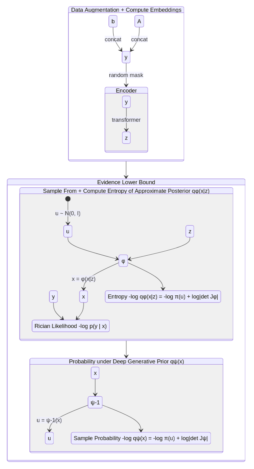
An encoder network $$$\mathcal{E}:\mathbb{R}_+^{n_{\mathrm{TE}}}\times\mathbb{R}_+^{n_{\mathrm{TE}}\times{}n_{T_2}}\rightarrow\mathbb{R}^{n_{\mathbf{z}}}$$$ is used to reduce $$$\mathbf{y}$$$ to $$$(n_{\mathbf{z}}=12)$$$-dimensional embeddings $$$\mathbf{z}=\mathcal{E}(\mathbf{y})$$$, i.e. $$$q_{\varphi}(\mathbf{x}|\mathbf{y})=q_{\varphi}(\mathbf{x}|\mathbf{z}=\mathcal{E}(\mathbf{y}))$$$. The three networks $$$\varphi(\mathbf{u};\mathbf{z}),\,\psi(\mathbf{u}),\,\mathcal{E}(\mathbf{y})$$$ are trained jointly using amortized variational inference^13,15-17 to minimize the following (negative) evidence lower bound (ELBO): $$\mathcal{L}_{\text{ELBO}}(\mathbf{y})=\underset{\mathbf{x}\sim{}q_{\varphi}(\mathbf{x}|\mathbf{z})}{\mathbb{E}}[-\log{}p(\mathbf{y}|\mathbf{x})-\log{}q_{\psi}(\mathbf{x})+\log{}q_{\varphi}(\mathbf{x}|\mathbf{z})]\quad\text{where}\quad\mathbf{z}=\mathcal{E}(\mathbf{y}).$$ Figure 1 illustrates how $$$\mathcal{L}_{\text{ELBO}}$$$ is computed.
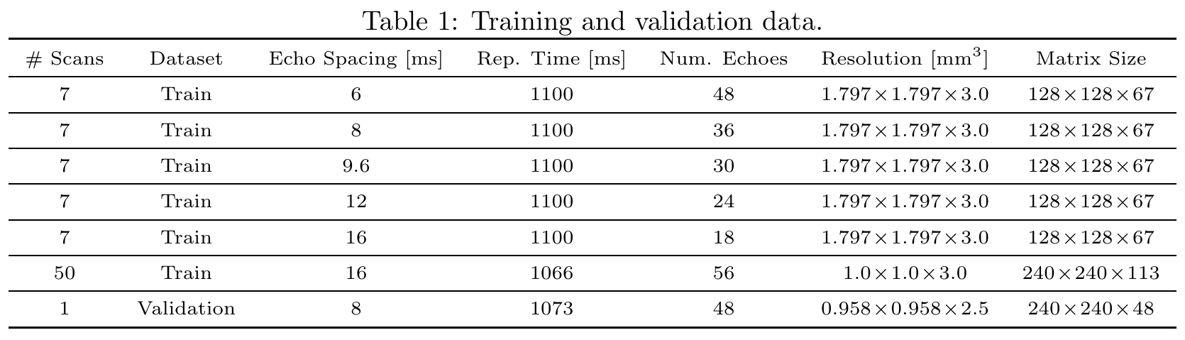
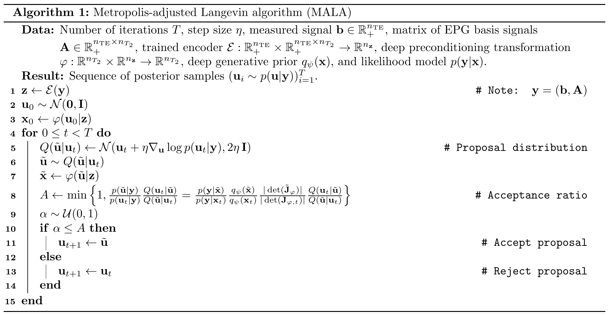
$$$\mathcal{E}$$$ consists of a 2-layer multilayer perceptron (MLP) (hidden dimension $$$512$$$, ReLU activation), a 2-layer transformer with multiheaded self-attention ($$$16$$$ heads, token size $$$128$$$), and another 2-layer MLP with output dimension $$$n_{\mathbf{z}}=12$$$; $$$\varphi(\mathbf{u};\mathbf{z})$$$ (similarly, $$$\psi(\mathbf{u})$$$) consists of $$$L=16$$$ (un)conditional linear coupling flows^18,19 interleaved with orthogonal linear flows. The Adam²⁰ optimizer is used with weight decay $$$\gamma=0.01$$$; initial learning rate $$$\eta=2\cdot{}10^{-4}$$$ decays to $$$\eta=10^{-7}$$$ following a cosine schedule; $$$500,\!000$$$ training steps are performed with mini-batches of $$$128\times{}(\mathbf{b},\mathbf{A})$$$ pairs; all $$$\mathbf{b},\mathbf{A}$$$ are padded with zeros to length $$$n_{\mathrm{TE}}=56$$$; data is augmented by random masking to length $$$16\le{}n_{\mathrm{TE}}\le{}56$$$; training/validation datasets are detailed in Table 1. After training, sampling $$$\mathbf{u}\sim{}p(\mathbf{u}|\mathbf{y})$$$ is performed via the Metropolis-adjusted Langevin algorithm (MALA); see Algorithm 1.

Results

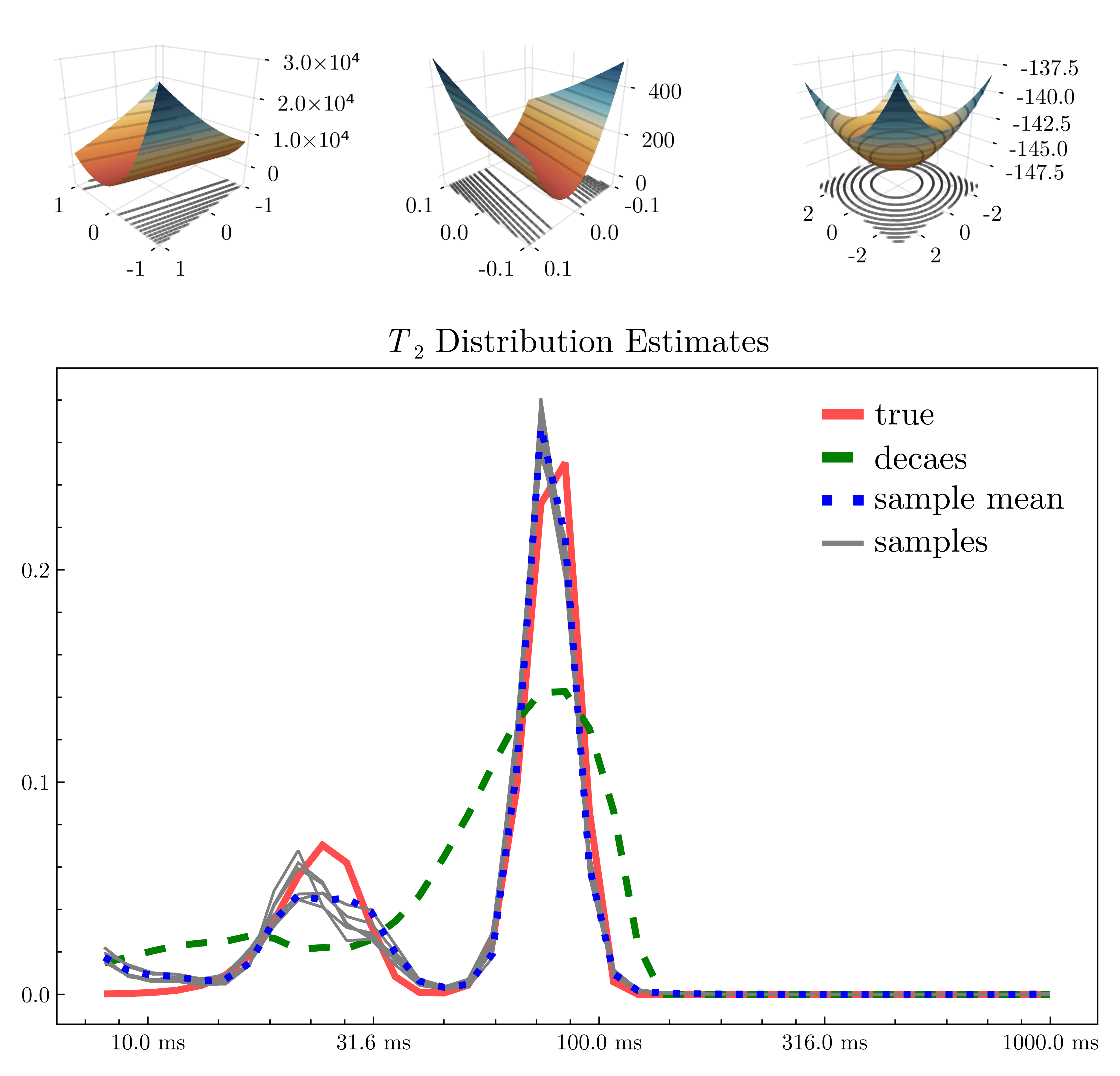
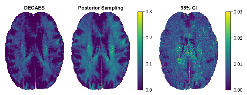
Figure 4 illustrates the posterior likelihood surface $$$-\!\log{}p(\mathbf{u}|\mathbf{y})$$$ in two random orthogonal directions before and after applying the learned preconditioning $$$\varphi$$$. The surface becomes more symmetric and well-conditioned, making exploration of the posterior space feasible. In lieu of a gold-standard method for comparison, in Figure 4 we compare NNLS with posterior sampling on a toy bimodal $$$T_2$$$-distribution corrupted with Rician noise ($$$\text{SNR}=50$$$). Posterior sampling both captures the peaks more faithfully, and illustrates the variety of plausible short peaks. Figure 5 compares MWF images on a validation image. MWF computed via MALA appears more spatially uniform, despite independent voxelwise sampling.

Discussion and conclusion

We have shown that posterior sampling over a learned manifold of $$$T_2$$$ distributions, aided by a deep generative prior, is feasible and indeed beneficial when compared with NNLS-based methods. Note that this does come at a cost: $$$T_2$$$ distributions significantly different than those seen during training will be avoided by the deep prior. We have not observed this issue, likely due to the size and diversity of the training set.

Acknowledgements

Natural Sciences and Engineering Research Council of Canada, Grant/Award Number 016-05371, the Canadian Institutes of Health Research, Grant Number RN382474-418628, the National MS Society (RG-1507-05301). J.D. is supported by NSERC Doctoral Award and Izaak Walton Killam Memorial Pre-Doctoral Fellowship. A.R. is supported by Canada Research Chairs 950-230363. This work was conducted on the traditional, ancestral, and unceded territories of Coast Salish Peoples, including the territories of the xwməθkwəy̓əm (Musqueam), Skwxwú7mesh (Squamish), Stó:lō and Səl̓ílwətaʔ/Selilwitulh (Tsleil-Waututh) Nations.