Synopsis

Keywords: Contrast Agent, DSC & DCE Perfusion

The conventional deconvolution method in DSC perfusion MRI suffers from sensitivity to noise and threshold level. Regularization methods to mitigate the noise issue also suffers from other issues. In this study, we present a deep learning approach to perform deconvolution more robustly and accurately. Our result showed multi layers perceptron (MLP) performed deconvolution more accurately in synthetic data compared to the traditional regularization method. We also showed that MLP performed more robustly in patient data with varying levels of noise. This study provides a strong argument for using MLP as a stable and accurate deconvolution method for DSC perfusion calculation.

Introduction

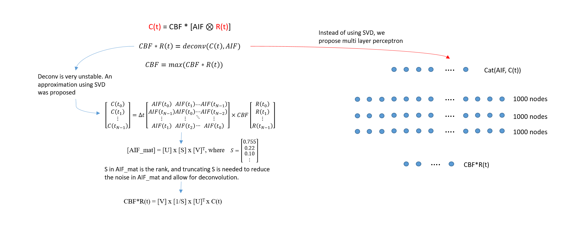
Calculation of perfusion parameters from dynamic susceptibility contrast (DSC) MRI data requires the use of deconvolution method, which calculates tissue-specific response function (Rt) from tissue concentration (Ct) and arterial input function (AIF). In practice, deconvolution is typically performed in DSC MRI using block-circulant singular value decomposition (cSVD) with truncation based on some threshold to reduce the effect of noise in AIF and Ct (1,2). Although the sensitivity to noise can be mitigated, the method still suffers from sensitivity to the choice of the threshold level (3). In this study, we propose a simulation-based deep learning approach to solving the deconvolution problem for more stable and accurate mapping of DSC perfusion parameters.

Method

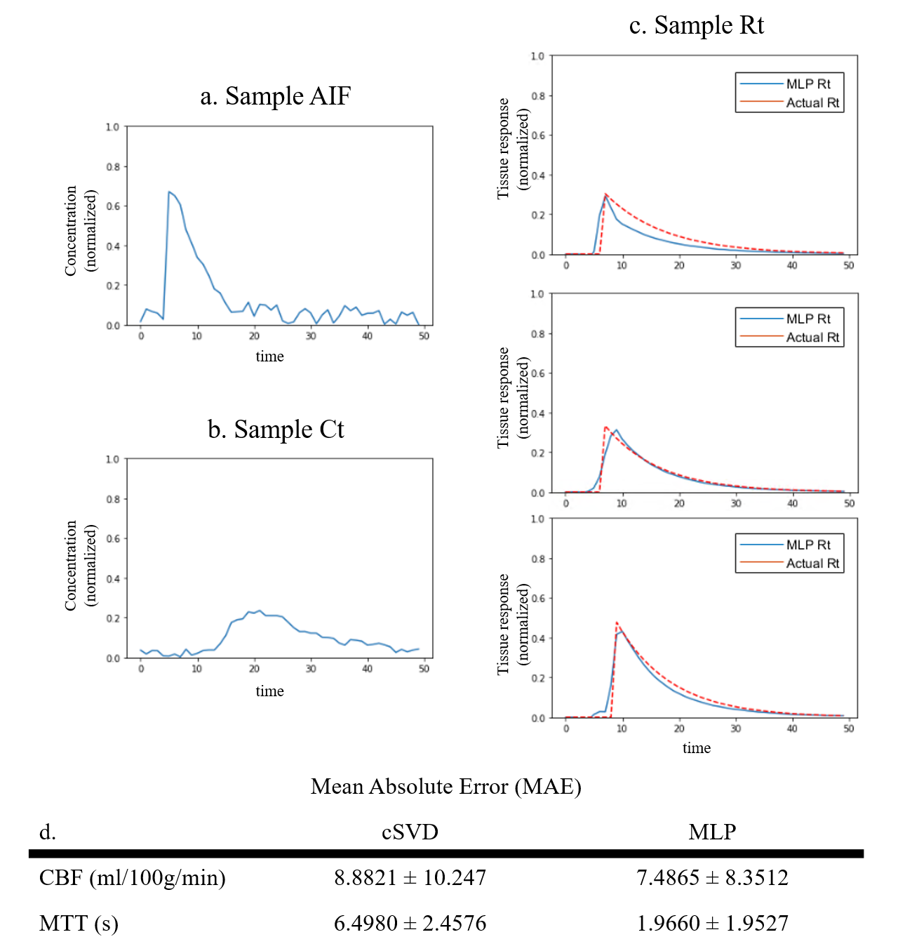
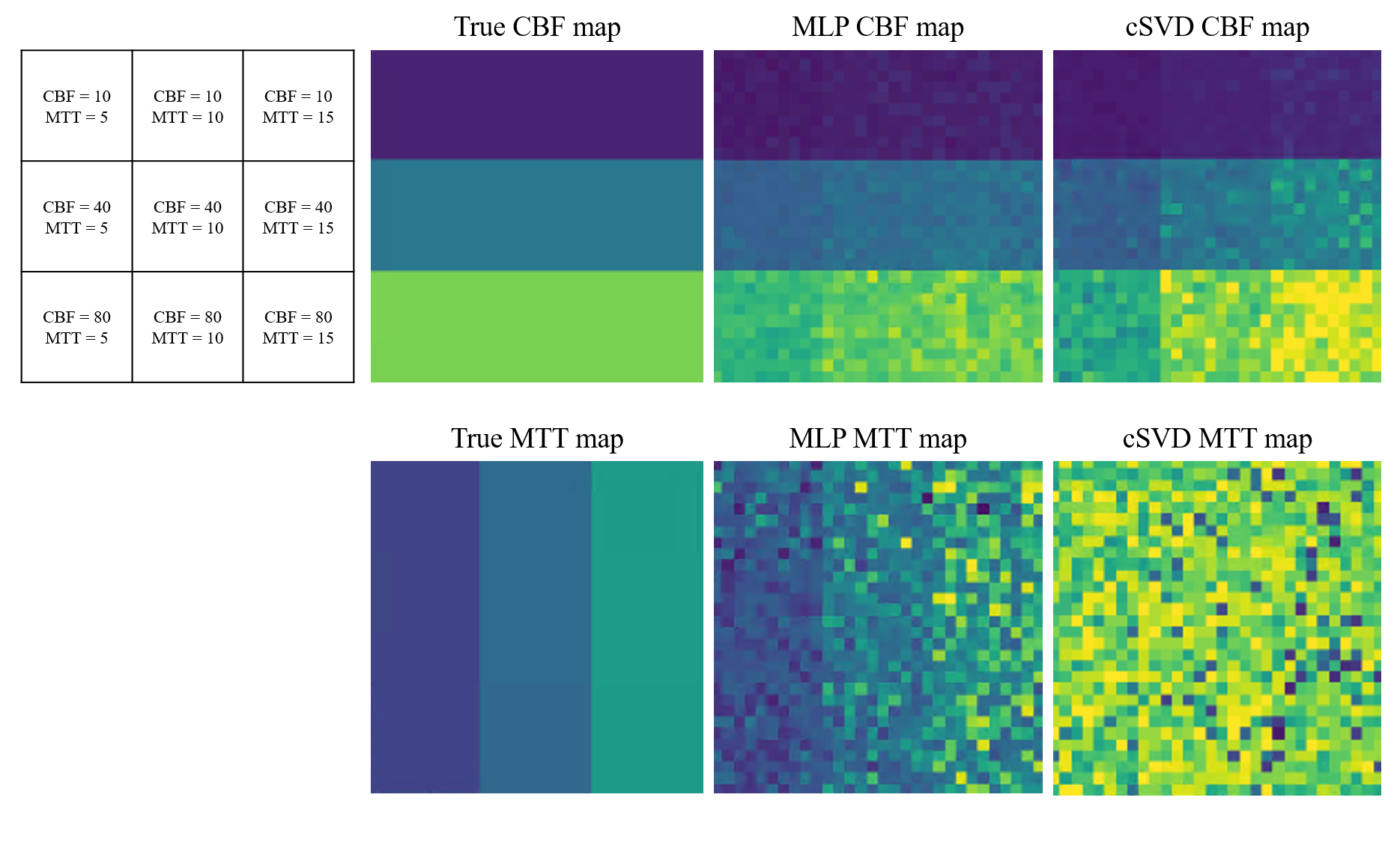
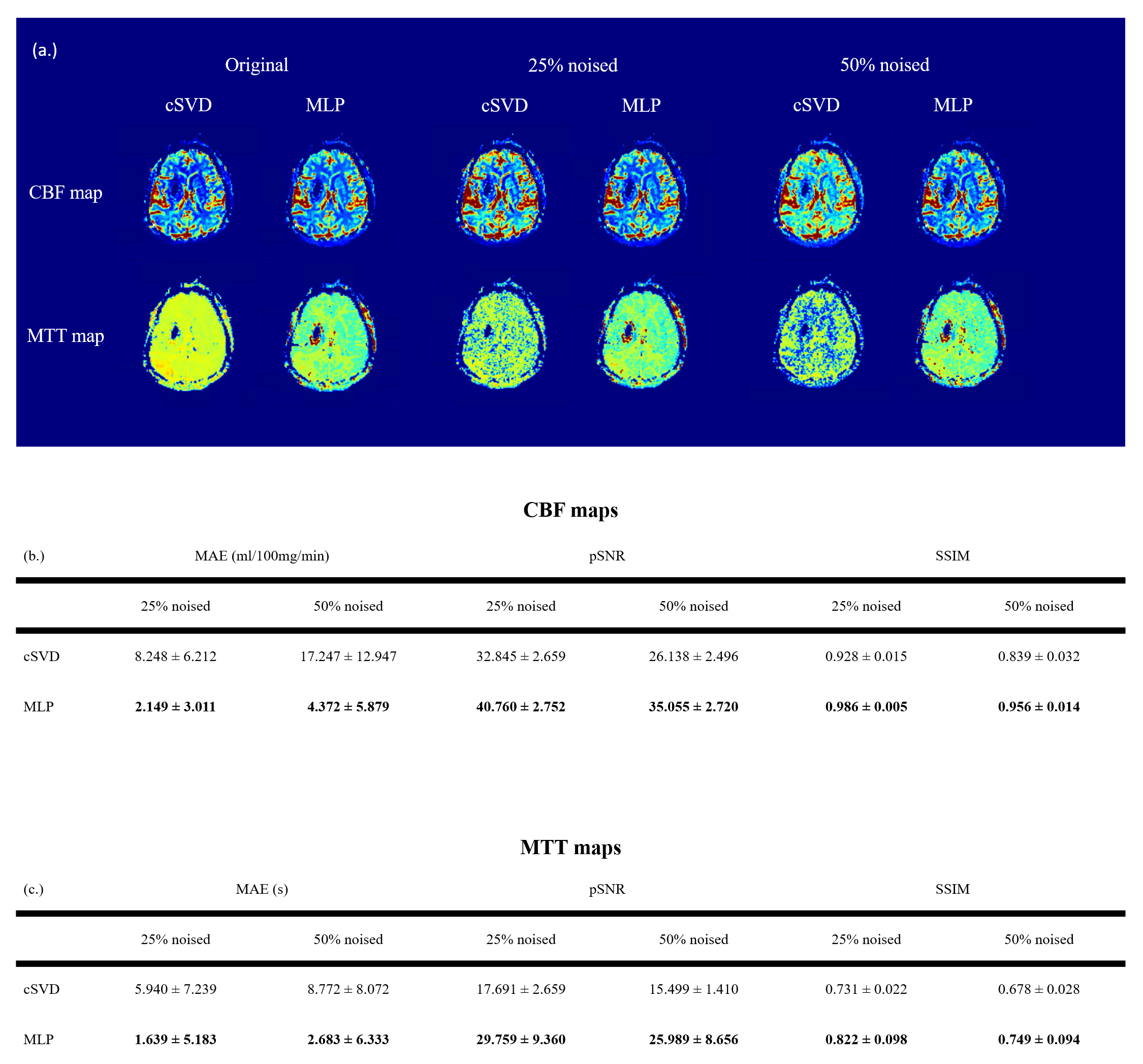
A synthetic DSC MRI time series with 50 time points were first created from a model AIF and Rt that are parameterized by MTT and CBF values (1,4). Then, Ct could be generated by simple AIF and Rt convolution. The AIF was designed to have 0-5s arrival delay while the Rt was designed to have another 0-10s delay before responding to AIF, reflecting the possible transit time from the AIF measurement site to the tissue location. CBF was varied from 0-70 ml/100g/min while MTT was varied from 0-15 sec which bounded the Rt to reasonable values. A random noise was introduced to slightly corrupt the AIF and Ct by 10% of their maximum before feeding them into the deep learning network.
A multi layers perceptron (MLP) network was designed to take AIF and Ct as input (100 nodes) and Rt as the output (50 nodes) with 3 layers of 1000 nodes each (figure 1). The MLP was trained purely on synthetic data to match the generated Rt with the actual Rt using L1loss. The MTT could be calculated as the full width at half maximum of Rt while CBF was calculated as the maximum of the Rt function. The generated Rt was further evaluated by numerically comparing the CBF and MTT values using the mean absolute error (MAE) and visually by generating CBF and MTT maps. The MLP application was further evaluated with real-world patient data where the MLP-generated CBF maps were compared to the CBF maps from cSVD deconvolution method. Three different levels of noise (0, 25%, and 50% of peak DSC MRI signal intensity) were added to the patient data to compare the robustness of the MLP and cSVD methods. Mean average error (MAE), peak signal-to-noise ratio (pSNR) and structural similarity (SSIM) between the CBF maps and MTT maps from original data versus noised data were calculated over 5 patients.

Results

Representative synthetic AIF, Ct, and MLP-generated Rt are shown in figure 2a-c. Three cases of the MLP generated Rt (figure 2c, blue line) showed good agreement with the actual Rt (figure 2c, red dashed line) in terms of the general shape and the peak height. The errors in CBF and MTT values estimated from the MLP and cSVD deconvolution methods are shown in the table (figure 2d). MLP provided more accurate CBF and MTT values than the cSVD deconvolution method (signed rank test, (P < 0.05)). A visual representation of CBF and MTT maps for various CBF and MTT values also showed a more stable CBF and MTT calculation when using MLP as opposed to cSVD (figure 3). For the patient data, the MLP method showed similar CBF and MTT maps compared to those of the cSVD method when no noise was added, however, the MLP method was much more robust than the cSVD method in the presence of noise (figure 4).

Discussion

The proposed MLP method showed a more stable result for deconvolution compared to the standard cSVD method when evaluated against synthetic DSC MRI time series. We believe this is partially due to the fact that the cSVD method is susceptible to noisy AIF and Ct. Furthermore, the choice of truncation in cSVD can vary largely on case-by-case basis. This is further demonstrated for the noise-corrupted patient data, where the CBF and MTT values from the cSVD method were significantly affected by the noise whereas those from the proposed MLP were mostly maintained and robust to the noise.

Conclusion

This study provides a deep learning alternative to the cSVD deconvolution method that is traditionally used in perfusion calculation of DSC MRI data. The MLP method showed better accuracy in synthetic DSC MRI data with varying combinations of CBF and MTT values compared to the cSVD method. While the MLP was trained using purely synthetic data, it performed well and more robust to the noise than the cSVD method in patient data, validating its application in real clinical environment. Cumulatively, these results provide a strong argument for using MLP as a more stable deconvolution method for DSC perfusion calculation in general.

Acknowledgements

No acknowledgement found.