Synopsis

Keywords: White Matter, Machine Learning/Artificial Intelligence

We present a novel framework for estimating microstructural parameters of compartment models using recently developed orientationally invariant spherical convolutional neural networks and efficiently simulated training data. The networks were trained to predict the ground-truth parameter values from simulated noisy data and applied on imaging data acquired in a clinical setting to generate microstructural maps. Our network could estimate model parameters more accurately than conventional non-linear least squares or a multi-layer perceptron applied on powder-averaged data (i.e., the spherical mean technique).

Introduction

We present a novel framework for estimating microstructural parameters of Gaussian compartment models using recently developed orientationally invariant spherical convolutional neural networks (sCNNs) by Esteves et al.¹ and efficiently simulated training data. The networks were trained to predict the ground-truth parameter values from simulated noisy data, and the trained models were applied to imaging data acquired in a clinical setting to generate microstructural maps.

Methods

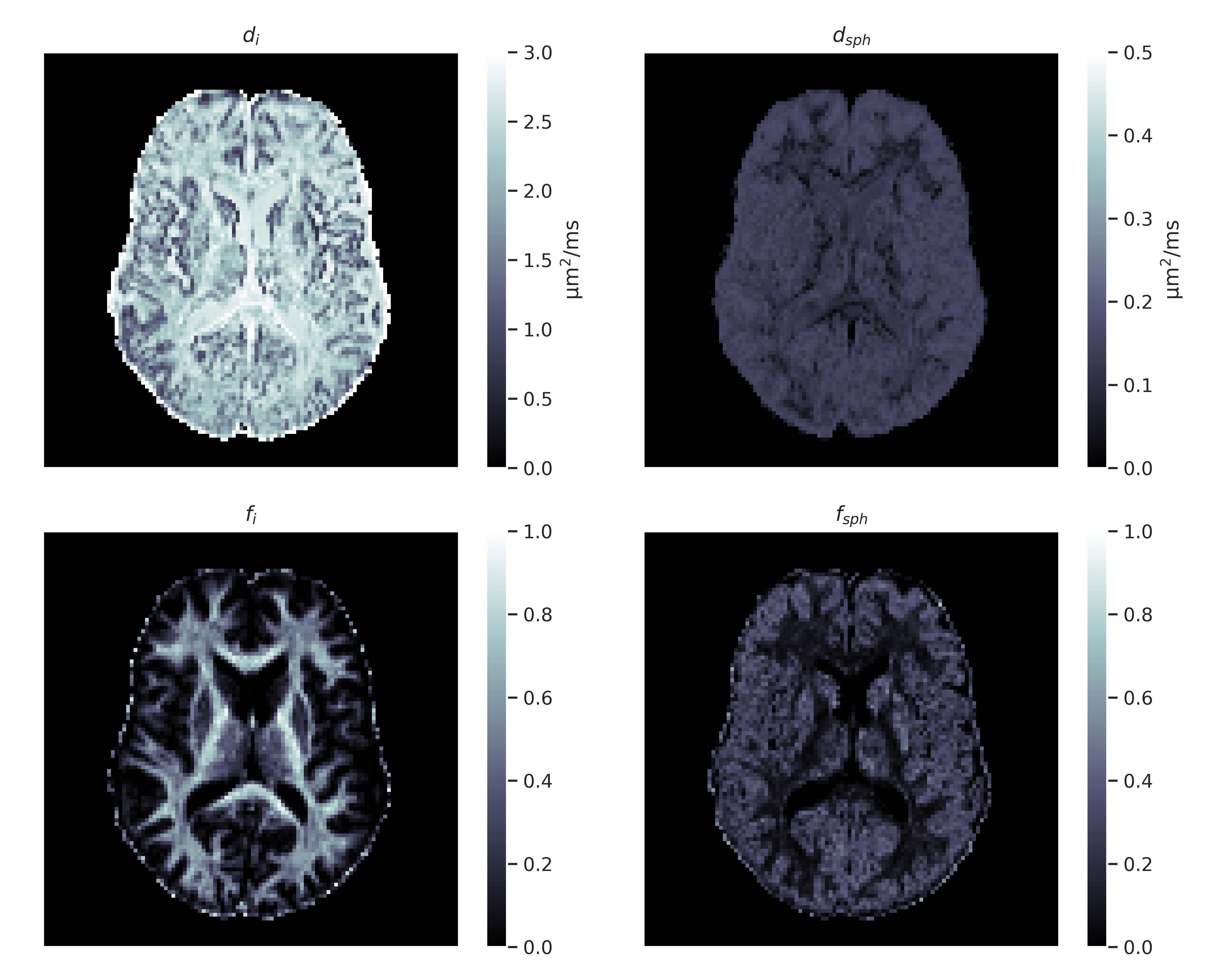
Imaging experiments: Four healthy adult volunteers were scanned on a Siemens Magnetom Prisma 3T. Data was denoised² and motion/distortion-corrected³. Signal-to-noise ratio (SNR) was estimated as the inverse of the standard deviation of the normalized signals with $$$b=0$$$. Three volunteers were scanned using a standard clinical high-angular resolution diffusion imaging (HARDI) protocol with non-zero b-values of 1 and 2.2 ms/µm² with 60 directions over half a sphere each. The total scan time was 7 minutes. Fibre orientation distribution functions (ODFs) were estimated with multi-tissue constrained spherical deconvolution⁴. One volunteer was scanned using tensor-valued diffusion encoding⁵. The acquisitions with linear b-tensors were performed with b-values of 0.5, 1, 2, 3.5, and 5 ms/µm² with 12, 12, 20, 20, and 30 directions over half a sphere. The acquisitions with planar b-tensors were performed with b-values of 0.5, 1, and 2 ms/µm² with 12, 12, and 20 directions over half a sphere. The total scan time was 12 minutes.

Microstructural models: We focused on a 2-compartment model by Kaden et al.⁶ that enables model parameters to be estimated from powder-averaged HARDI data using non-linear least squares (NLLS). The model contains two parameters: intra-neurite signal fraction $$$f$$$ and diffusivity $$$d$$$. We also estimated the parameters of a 3-compartment model by Gyori et al.⁷ that enables apparent neural soma density imaging using tensor-valued diffusion encoding. The model contains four parameters: intra-neurite signal fraction $$$f_\text{i}$$$, spherical compartment signal fraction $$$f_\text{sph}$$$, intra-neurite diffusivity $$$d_\text{i}$$$, and spherical compartment diffusivity $$$d_\text{sph}$$$.

Simulations: Signal was represented as a spherical convolution of an ODF by a microstructural kernel response function $$$K$$$: $$S(\mathbf{\hat{n}})=\int_{\mathbf{R}\in\text{SO}(3)}d\mathbf{R}\ \text{ODF}(\mathbf{R}\mathbf{\hat{e}_3}) K(\mathbf{R}^{-1}\mathbf{\hat{n}}).$$ The above equation was evaluated as a point-wise product in the spherical harmonics domain using the spherical convolution theorem⁸. Kernel response function values were computed as $$K(\mathbf{\hat{n}})=\sum_i f_i\exp(-\mathbf{b}:\mathbf{D}_i),$$ where $$$f_i$$$ is the signal fraction of the $$$i$$$th compartment, $$$\mathbf{b}$$$ is the b-tensor corresponding to $$$\mathbf{\hat{n}}$$$ and a b-value equal to $$$\text{Tr}(\mathbf{b})$$$, and $$$\mathbf{D}_i$$$ is a diffusion tensor corresponding to the $$$i$$$th compartment. Rician noise was added to the signals with an SNR matching that of the imaging data (SNR = 30 for HARDI data and SNR = 20 for tensor-valued data).

Network architecture: The sCNN consisted of three spherical convolution layers¹ with 16, 32, and 64 output layers followed by global pooling and three fully connected layers with a hidden layer size of 128. The number of input channels was equal to the number of shells in the data and the number of outputs was equal to the number of predicted parameters. For comparison, an MLP with three hidden layers of 256 nodes each was trained to predict the model parameters from powder-averaged data. Non-linearities were rectified linear units (ReLUs) and each hidden fully connected layer was followed by batch normalization.

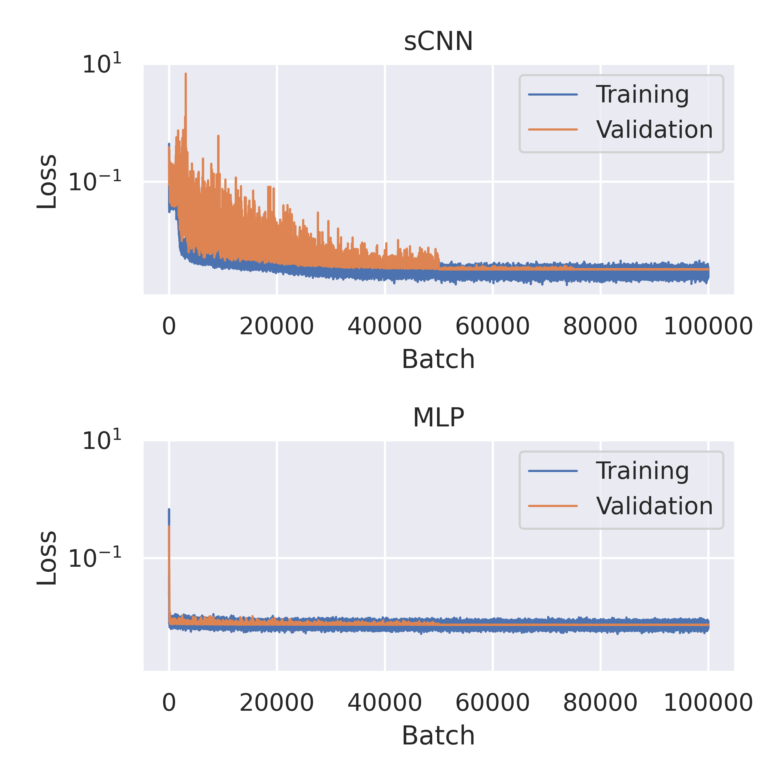
Training: The models were trained over $$$10^5$$$ batches of simulated data generated during training. Each batch contained signals from $$$10^3$$$ microstructural configurations produced by random sampling. ODFs were sampled from one of the volunteers, normalized, and randomly rotated. $$$f\sim\text{U}(0,1)$$$, $$$d\sim\text{U}(0,3$$$ µm²/ms$$$)$$$, $$$f_\text{i}\sim\text{U}(0,1)$$$, $$$f_\text{sph}\sim\text{U}(0,f_\text{i})$$$, $$$d_\text{i}\sim\text{U}(0,3$$$ µm²/ms$$$)$$$, and $$$d_\text{sph}\sim\text{U}(0,\text{max}(d_\text{i}, 0.5$$$ µm²/ms$$$))$$$. The upper limit of $$$d_\text{sph}$$$ was chosen to correspond to a sphere with a diameter of 25 µm using the Monte Carlo simulator Disimpy⁹. Validation and test datasets were constructed similarly, except that they contained $$$10^5$$$ and $$$10^6$$$ microstructural configurations, respectively, and the ODFs were sampled from different subjects. Networks were trained with ADAM and an initial learning rate of $$$10^{-3}$$$, which was reduced by 90% at batches $$$5\cdot 10^4$$$ and $$$7.5\cdot 10^4$$$. Mean squared error (MSE) was used as the loss function, and the diffusivity parameters were scaled by $$$\frac{1}{3}$$$ so that they would range from 0 to 1 like the signal fractions. Training the sCNNs took 7 h on NVidia's Tesla T4 with 16 GB of memory.

Results​

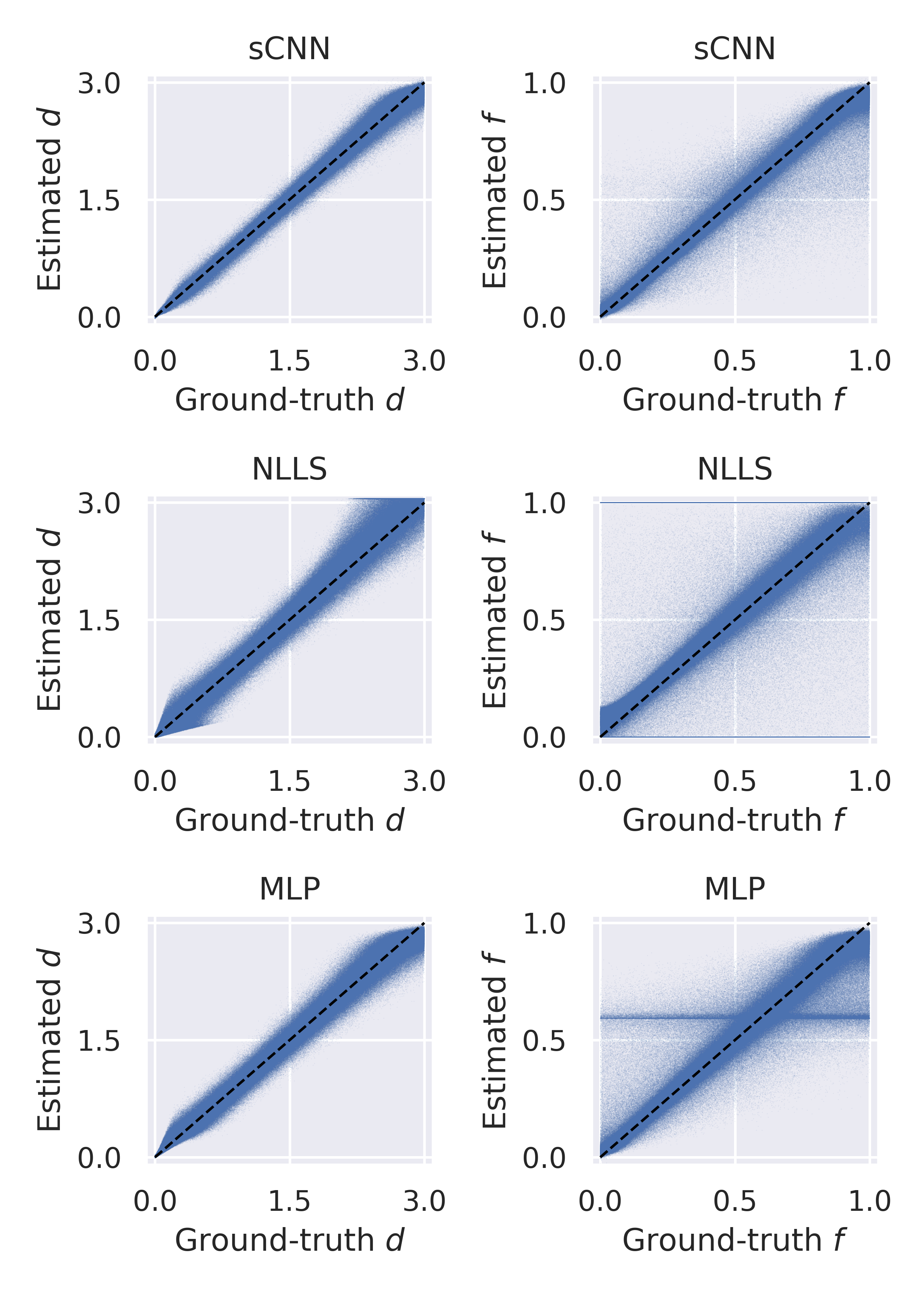
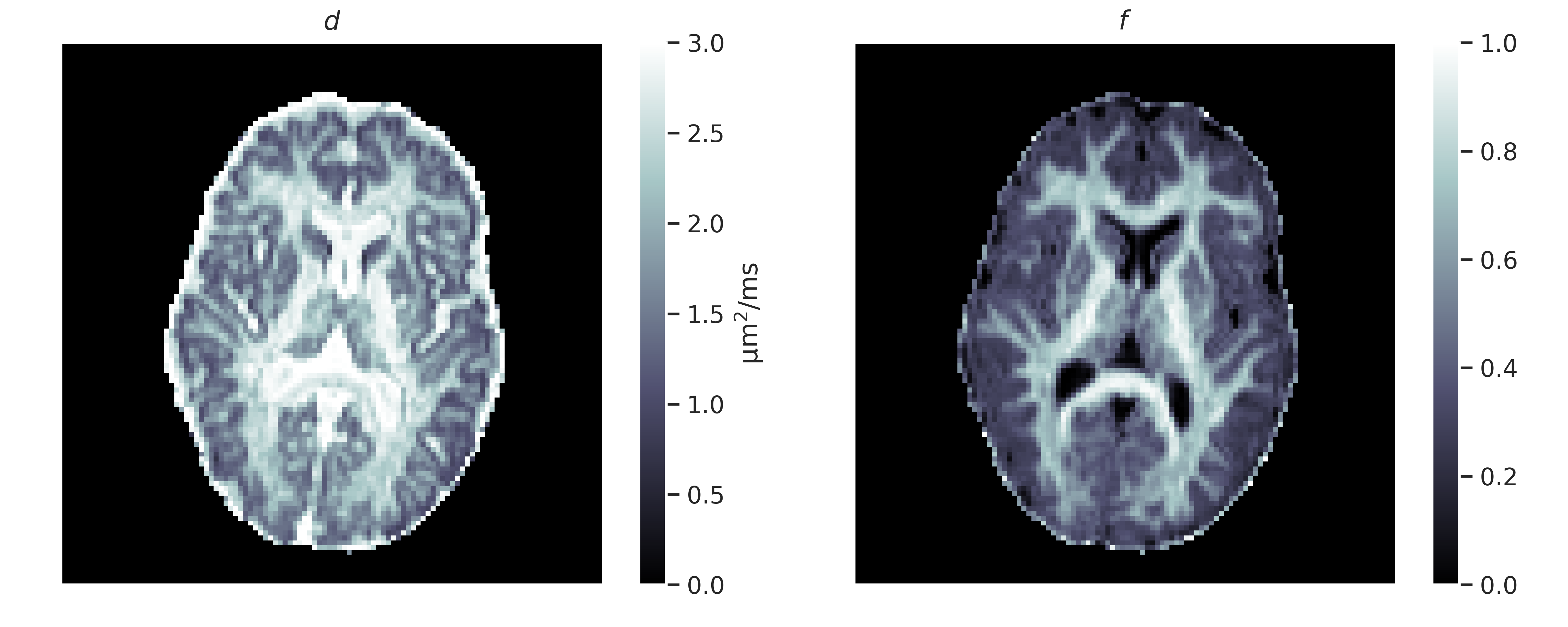
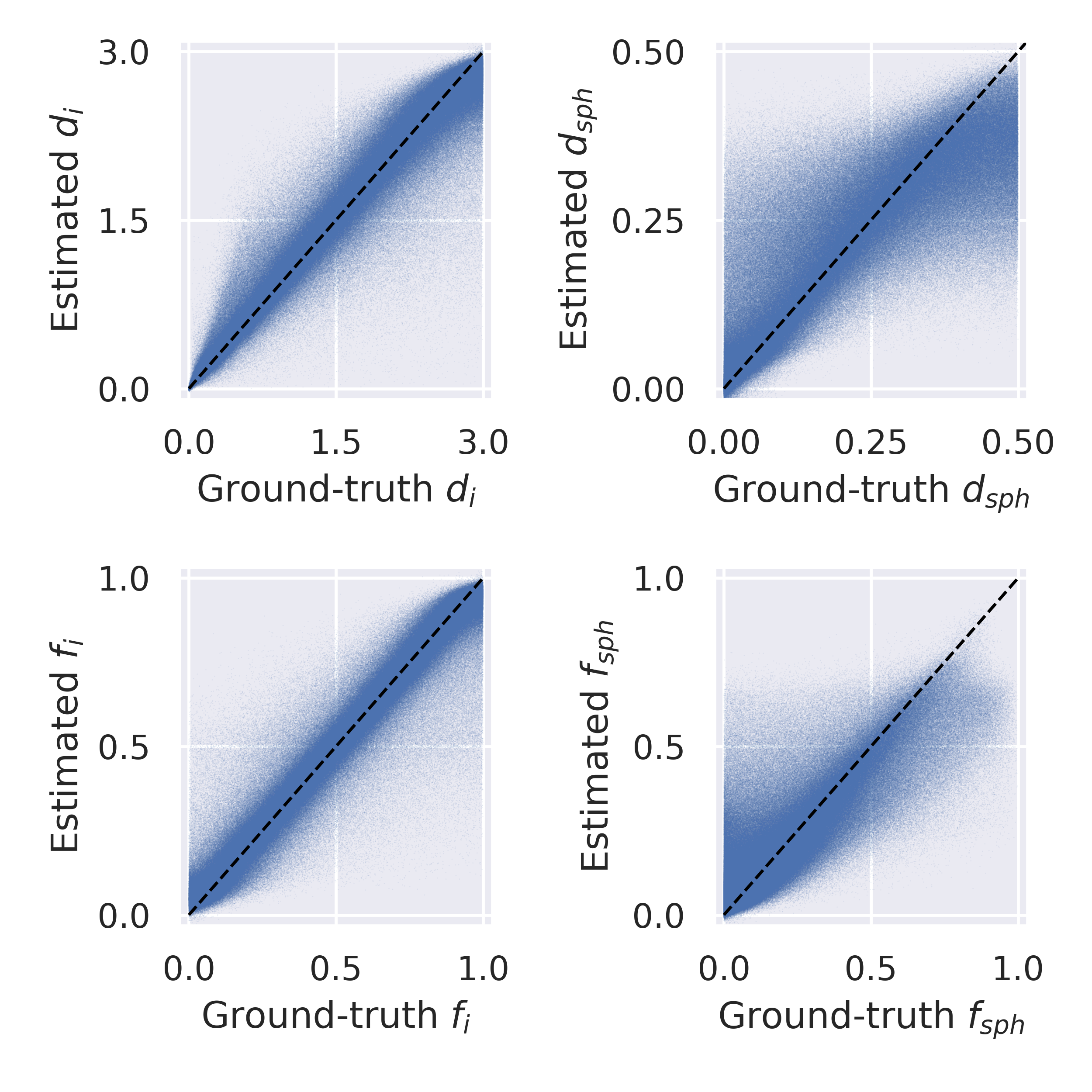
The sCNN outperformed NLLS and the MLP. Mean squared error (MSE) of $$$d$$$ was $$$0.76\cdot 10^{-2}$$$ µm²/ms for sCNN, $$$3.01\cdot 10^{-2}$$$ µm²/ms for NLLS, and $$$1.54\cdot 10^{-2}$$$ µm²/ms for MLP. MSE of $$$f$$$ was $$$0.52\cdot 10^{-2}$$$ for sCNN, $$$3.75\cdot 10^{-2}$$$ for NLLS, and $$$1.27\cdot 10^{-2}$$$ for MLP. MSE of $$$d_\text{i}$$$ was $$$7.52\cdot 10^{-2}$$$ µm²/ms for sCNN and $$$10.20\cdot 10^{-2}$$$ µm²/ms for MLP. MSE of $$$d_\text{sph}$$$ was $$$0.83\cdot 10^{-2}$$$ µm²/ms for sCNN and $$$0.94\cdot 10^{-2}$$$ µm²/ms for MLP. MSE of $$$f_\text{i}$$$ was $$$0.83\cdot 10^{-2}$$$ for sCNN and $$$1.89\cdot 10^{-2}$$$ for MLP. MSE of $$$f_\text{sph}$$$ was $$$1.59\cdot 10^{-2}$$$ for sCNN and $$$2.29\cdot 10^{-2}$$$ for MLP. As expected based on previous work^7,10, estimation of $$$d_\text{sph}$$$ and $$$f_\text{sph}$$$ was difficult, especially for low $$$f_\text{sph}$$$. Whole-brain microstructural maps were generated by the sCNN within seconds on the GPU.

Conclusion

sCNNs can improve the accuracy of microstructural parameter estimation and provide a compelling alternative to estimating parameters from powder-averaged data.

Acknowledgements

No acknowledgement found.