2628
Myelin water fraction mapping using relaxation spectra from steady-state gradient echo imaging with partial RF spoiling1German Center for Neurodegenerative Diseases (DZNE), Bonn, Germany, 2Department of Physics & Astronomy, University of Bonn, Bonn, Germany
Synopsis
Keywords: White Matter, Modelling, Myelin
A new approach for myelin water fraction (MWF) mapping is presented, based on gradient echo signals with small RF spoiling phase increments. Partially spoiled gradient echo data with 20 different phase increments ($$$|\Delta\phi|\le20^\circ$$$) were efficiently acquired with a custom skipped-CAIPI 3D-EPI sequence. The data is well-suited for a novel joint-fitting approach of $$$T_1$$$- and $$$T_2$$$-spectra, from which high-quality whole-brain MWF maps are derived. MWF-maps show qualitatively good agreement with published data in the white matter (WM). Additionally, the approach seems to provide robust estimates in regions with small MWF, such as the gray matter (GM).Introduction
The myelin content can be approximated by the amount of myelin water (MW), which is trapped in the myelin sheath. MW has shorter relaxation times than surrounding axonal and extracellular water (AEW)1. The concentration ratio of MW over MW+AEW defines the myelin water fraction (MWF), which can be derived from relaxation spectra. Common approaches employ multi-exponential fitting of multi-echo MRI data using either spin-echoes2 or gradient-echoes3. The robustness of these methods is limited, since only few echoes at short echo times are sensitive to the MW component. Additionally, multi-exponential data fitting is an ill-posed inverse problem4. Thus, data fitting is often unstable, especially in regions with low MW content5. Alternatively, a steady-state gradient echo (GRE) sequence with short TR and small RF spoiling phase increment (partial spoiling) is sensitive to changes of relaxation times6. It was previously shown that $$$T_2$$$ can be robustly estimated from phase images of two GRE acquisitions with small and opposite phase increments7. We propose to jointly estimate $$$T_1$$$ and $$$T_2$$$ spectra from magnitude and phase data of such partially spoiled GRE acquisitions with varying phase increments. The approach is sensitive to MW and AEW components and the inversion results in robust MWF estimates.Methods
TheoryThe complex GRE signal with magnitude $$$a$$$ and phase $$$\theta$$$ is defined as $$ s(T_1,T_2;\alpha,TR,\Delta\phi) \equiv a\exp[\text{i}\theta]\;,$$ where $$$(T_1,T_2)$$$ are the longitudinal and transverse relaxation times and $$$(\alpha,TR,\Delta\phi)$$$ are the flip-angle, repetition time, and RF spoiling increment of the GRE sequence, respectively. We assume that the GRE signal within an imaging voxel results from isochromate-superposition of static $$$T_1$$$ and $$$T_2$$$ spectra, $$$w(T_1)$$$ and $$$w(T_2)$$$. Furthermore, we assume a voxel-specific linear relationship between the relaxation times, $$$T_1=\eta T_2$$$, i.e. the $$$T_1$$$-spectrum is a stretched version of the $$$T_2$$$-spectrum, $$$w(T_1)=w(\eta T_2)$$$. Under these assumptions, the GRE signal (at echo time zero) is given by $$s_{w,\eta}({\Delta\phi,\alpha})=\int_0^{\infty}{w(T_2)}s({\eta}T_2,T_2;TR,\Delta\phi,\alpha)\;\text{d}T_2\;.$$ After discretization to column vectors,
$${\bf{T_2}}=[T_{2,1},...,T_{2,N}]^T,\;{\bf{w}}=[w_1,...,w_N]^T,\;{\bf{\Delta\phi}}=[\Delta\phi_1,...,\Delta\phi_M]^T,\;{\bf{s}}=[s_1,...,s_M]^T$$ we estimate the $$$T_2$$$-spectrum, $$${\bf{w}}$$$, and the $$$T_1$$$-over-$$$T_2$$$ ratio, $$$\eta$$$, for each voxel by solving the regularized, underdetermined ($$$M<N$$$) optimization problem
$$\underset{{\bf{w}},\eta}{\text{min}}\|{\bf{S}}_{\eta,\alpha}\cdot{\bf{w}}-{\bf{\hat{s}}_{\alpha_a}}\|^2+\beta^2\|{\bf{w}}\|^2\;,$$
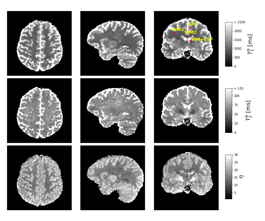
where $$$\beta$$$ is the regularization parameter, $$${\bf{\hat{s}}}_{\alpha_a}$$$ is the acquired data at an actual flip-angle $$$\alpha_a$$$, and $$${\bf{S}}_{\eta,\alpha}$$$ is a set of pre-computed $$$M\times{N}$$$ system matrices for suitable ranges of $$$\alpha$$$ and $$$\eta$$$ and fixed $$$TR$$$. After normalizing the solution $$$\bf{w}$$$, such that $$$\sum_{n=1}^N w_n=1$$$, the estimated MWF is given by $$MWF=\sum_{n=1}^{N_{MW}}w_n\quad\text{with}\quad{N_{MW}<N}\;,$$ where $$$T_{2,N_{MW}}\equiv{T_2}^{thresh}$$$ denotes an upper threshold for the MW component. For validation, we also compute the bulk $$$T_1$$$ and $$$T_2$$$ per voxel from the first moment of the normalized $$$T_2$$$-distribution, $$$\bf{w}$$$, and the estimated $$$T_1$$$-over-$$$T_2$$$ ratio, $$$\eta$$$: $$ T_1^{b}=\eta\,T_2^{b}=\eta\;{\bf{T_2}}^T\cdot{\bf{w}}\;.$$
Data acquisition
Single-subject data was collected on a 3 Tesla Siemens Skyra MRI scanner with a 32-ch-Rx head-coil (Siemens Healthineers, Erlangen). Whole-brain GRE data was efficiently acquired utilizing a skipped-CAIPI 3D-EPI sequence8 with an EPI-factor of 4, four-fold 2D-CAIPI acceleration, TE=3.5 ms, TR=9.5 ms, matrix size (Nx,Ny,Nz)=(150,150,118), isotropic resolution of 1.5 mm, and flip-angle $$$\alpha$$$=20$$$^\circ$$$; the latter provides a good compromise for MW and AEW signals. 20 repetitions with varying phase increment were acquired: $${\bf{\Delta\phi}}=[\pm{1}^\circ,\pm{2}^\circ,\pm{3}^\circ,\pm{4}^\circ,\pm{5}^\circ,\pm{6}^\circ,\pm{8}^\circ,\pm{11}^\circ,\pm{15}^\circ,\pm{20}^\circ].$$ The total acquisition time was 7:35 min. Additionally, a 3DREAM9 sequence was acquired, providing an actual flip-angle map. Before data fitting, the following processing steps were performed: Marchenko-Pastur PCA denoising (dwidenoise/mrtrix3), motion correction (mcflirt/FSL) of the complex data, background phase removal from the matching $$$\pm\Delta\phi$$$ phase images6, and brain extraction (bet/FSL).
Data fitting
The 4D set of GRE signals, $$${\bf{S}}_{\eta,\alpha}$$$, was precomputed utilizing extended phase graphs10 for all acquired $$$\bf{\Delta\phi}$$$, and on equidistant grids for $$$T_2$$$=[1,2,...,250] ms, $$$\eta$$$=[1.00,1.25,...,30.00], and $$$\alpha$$$=[16.00$$$^\circ$$$,16.25$$$^\circ$$$,...,24$$$^\circ$$$]. For each voxel, a 3D subset $$${\bf{S}}_{\eta,\alpha_n}$$$ is chosen, where $$$\alpha_n$$$ is closest to the measured flip-angle. The optimization problem is solved for $$$\bf{w}$$$ with non-negative least squares (NNLS)11, and the cost function error is minimized with respect to $$$\eta$$$ using scalar function minimization12. From the results $$$({\bf{w}},\eta)$$$ for all voxels, the MWF map is computed using $$$T_2^{thresh}$$$=35ms.4 Also, $$$T_1^b,T_2^b$$$ and $$$\eta$$$ maps are computed.
Results
FFig. 1A) shows that GRE signals with varying RF spoiling increment are highly sensitive to the relaxation times of MW and AEW. Axial slices of the in vivo data (Fig. 1B), emphasize the variation of magnitude and phase contrast. Fig. 2 depicts the resulting MWF maps, which show stable results already for small regularization parameters $$$\beta$$$. Fig. 3 shows estimates of relaxation time spectra from several voxels in different brain regions. MWF is highest for the voxel in the corpus callosum ("WM2"), and lowest for the GM-voxel. Finally, Fig. 4 depicts the bulk $$$T_1,T_2$$$ and $$$\eta$$$ maps.Discussion
The novel MWF-mapping approach utilizes joint $$$T_1$$$-$$$T_2$$$-spectra fitting of GRE signals with varying phase increment. MWF patterns in white matter agree well published findings1-5. We also observe robust estimates in regions with small MWF, such as gray matter. In contrast to multi-echo approaches, the MW signal fraction substantially contributes to all data points and benefits from short TR, since shorter $$$T_1$$$ reduces saturation compared to AEW. Also, the distinct MW/AEW signal shapes seem to reduce the ill-posedness of the optimization problem. However, we have not yet investigated the validity of the underlying model (static relaxation spectra with scaling $$$\eta$$$). Also, estimate biases due to exchange and $$$T_2^*$$$ need to be addressed.Acknowledgements
This work received financial support from the Helmholtz Association Initiative and Networking Fund, funding code ZT-I-PF-4-006 (Helmholtz Imaging Project "JIMM").References
1. Cornelia Laule, Irene M. Vavasour, Shannon H. Kolind, David K B Li, Tony L. Traboulsee, G. R Wayne Moore, and Alex L. MacKay. “Magnetic Resonance Imaging of Myelin.” Neurotherapeutics 4, no. 3 (2007): 460–84. https://doi.org/10.1016/j.nurt.2007.05.004.
2. Alex Mackay, Kenneth Whittall, Julian Adler, David Li, Donald Paty, and Douglas Graeb. “In Vivo Visualization of Myelin Water in Brain by Magnetic Resonance.” Magnetic Resonance in Medicine 31, no. 6 (June 1994): 673–77. https://doi.org/10.1002/mrm.1910310614.
3. Yiping P. Du, Renxin Chu, Dosik Hwang, Mark S. Brown, Bette K. Kleinschmidt-DeMasters, Debra Singel, and Jack H. Simon. “Fast Multislice Mapping of the Myelin Water Fraction Using Multicompartment Analysis Of T2* Decay at 3T: A Preliminary Postmortem Study.” Magnetic Resonance in Medicine 58, no. 5 (November 2007): 865–70. https://doi.org/10.1002/mrm.21409.
4. Eva Alonso-Ortiz, Ives R. Levesque, and G. Bruce Pike. “MRI-Based Myelin Water Imaging: A Technical Review: MRI-Based Myelin Water Imaging.” Magnetic Resonance in Medicine 73, no. 1 (January 2015): 70–81. https://doi.org/10.1002/mrm.25198.
5. Jongho Lee, Jae Won Hyun, Jieun Lee, Eun Jung Choi, Hyeong Geol Shin, Kyeongseon Min, Yoonho Nam, Ho Jin Kim, and Se Hong Oh. “So You Want to Image Myelin Using MRI: An Overview and Practical Guide for Myelin Water Imaging.” Journal of Magnetic Resonance Imaging, 2020, 1–14. https://doi.org/10.1002/jmri.27059.
6. Oliver Bieri, Klaus Scheffler, Goetz H Welsch, Siegfried Trattnig, Tallal C Mamisch, and Carl Ganter. “Quantitative Mapping of T2 Using Partial Spoiling.” Magnetic Resonance in Medicine 66, no. 2 (March 2011): 410–18. https://doi.org/10.1002/mrm.22807.
7. Xiaoke Wang, Diego Hernando, and Scott B. Reeder. “Phase‐based T2 Mapping with Gradient Echo Imaging.” Magnetic Resonance in Medicine 84, no. 2 (August 2020): 609–19. https://doi.org/10.1002/mrm.28138.
8. Rüdiger Stirnberg, and Tony Stöcker. “Segmented K‐space Blipped‐controlled Aliasing in Parallel Imaging for High Spatiotemporal Resolution EPI.” Magnetic Resonance in Medicine 85, no. 3 (March 2021): 1540–51. https://doi.org/10.1002/mrm.28486.
9. Philipp Ehses, Daniel Brenner, Rüdiger Stirnberg, Eberhard D. Pracht, and Tony Stöcker. “Whole-Brain B1-Mapping Using Three-Dimensional DREAM.” Magnetic Resonance in Medicine 82, no. 3 (2019): 924–34. https://doi.org/10.1002/mrm.27773.
10. Klaus Scheffler. “A Pictorial Description of Steady-States in Rapid Magnetic Resonance Imaging.” Concepts in Magnetic Resonance 11, no. 5 (1999): 291–304. https://doi.org/10.1002/(SICI)1099-0534(1999)11:5<291::AID-CMR2>3.0.CO;2-J.
11. scipy.optimize.nnls https://docs.scipy.org/doc/scipy/reference/generated/scipy.optimize.nnls.html
12. scipy.optimize.minimize_scalar https://docs.scipy.org/doc/scipy/reference/optimize.minimize_scalar-bounded.html
Figures
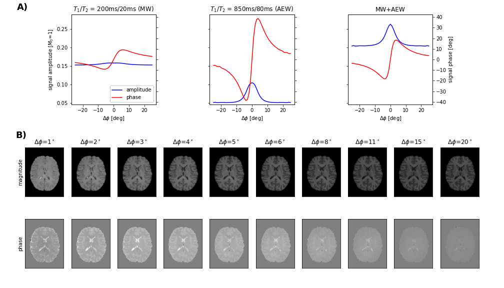
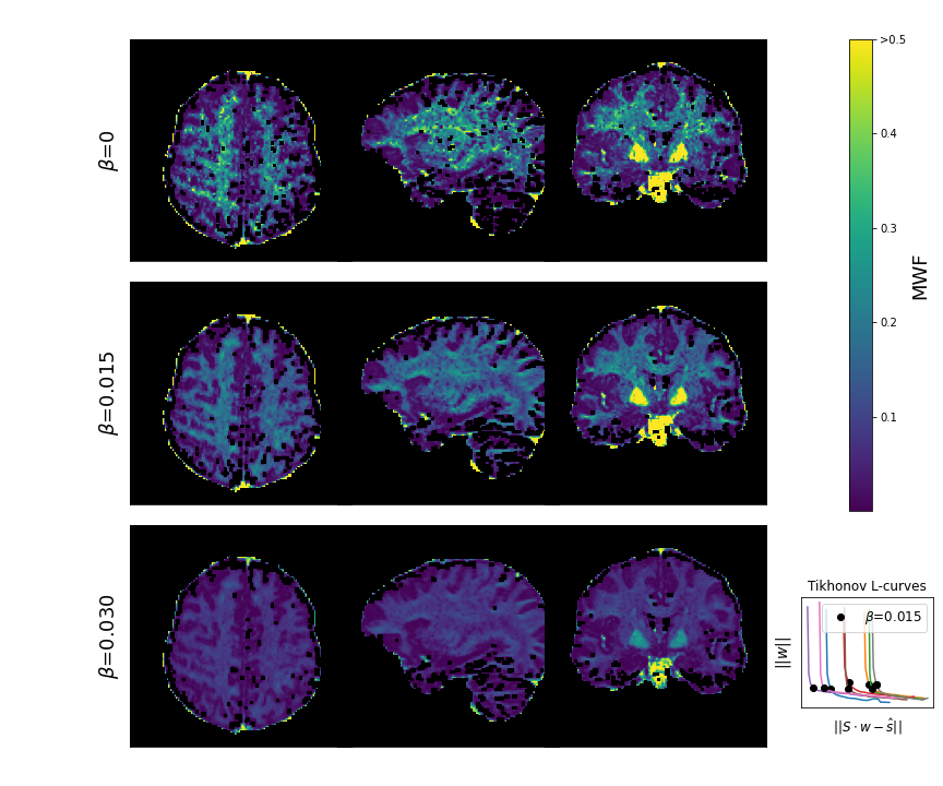
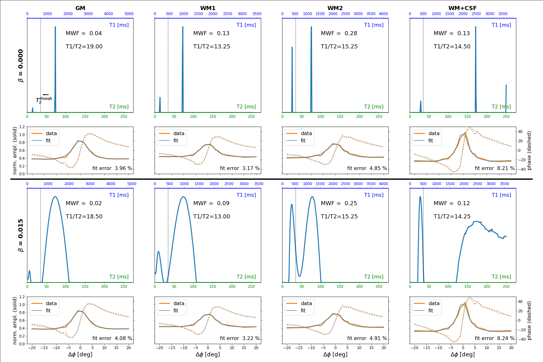
Figure 3: Example fit results for a voxel in GM (1st column), two voxels in WM (2nd and 3rd column), and a "partial-volume-voxel" in WM and CSF (last column). Upper and lower half of the plot show the estimated relaxation spectra and corresponding GRE signals (data and fit) without regularization (β=0) and with regularization (β=0.015), respectively. Note the different scaling of the spectra's T1-axes due to different estimates of η=T1/T2. The voxel locations are shown in Fig. 4.