2541
Impact of B0 field imperfections correction on BOLD sensitivity in 3D-SPARKLING fMRI data1Université Paris-Saclay, CEA, NeuroSpin, CNRS, Gif-sur-Yvette, France, 2Université Paris-Saclay, Inria, MIND, Palaiseau, France, 3Siemens Healthineers, Saint-Denis, France, 4Skope Magnetic Resonance Technologies AG, Zurich, Switzerland
Synopsis
Keywords: Data Acquisition, fMRI
Static and dynamic ∆B0 field imperfections are detrimental for fMRI applications as they degrade the temporal SNR (tSNR) and the sensitivity to the BOLD contrast. In this work we propose an experimental protocol for field imperfection monitoring and correction on 3D-SPARKLING fMRI data using the Skope Clip-on field camera in an alternative setting challenging its long TR constraint. We demonstrate the viability of our protocol and the reproducible gain in image quality, tSNR and retinotopic maps when correcting static and dynamic field imperfections on resting-state and task-based fMRI data for 3 healthy volunteersIntroduction
3D-SPARKLING1 is a novel non-Cartesian compressed sensing acquisition pattern recently assessed for high spatial resolution fMRI2. Similarly to its competitors, $$$\Delta\textrm{}B_{0}$$$ imperfections affect 3D-SPARKLING data and cause BOLD sensitivity loss. Correcting field imperfections can be performed during image reconstruction given estimates of static inhomogeneities and their dynamic fluctuations3. A novel technology based on NMR probes4,5 that allows us to monitor field fluctuations concurrently to the imaging process has been gaining ground over the last years6–8. However, the minimal TRprobe required by this system is constrained by the $$$T_{1}$$$ relaxation time of the NMR-active product used and must be quite long to avoid residual magnetization between the consecutive shots. This is hardly achievable in a realistic 3D fMRI scenario where TRprobe=TRshot. The authors of8 managed to use this system to acquire realistic 3D fMRI data with a short TRshot and a long TRprobe: They assumed repeatable readouts between the shots, skipped monitoring some shots and interpolated the missing data. Such a strategy is impractical for 3D-SPARKLING applications given the random nature of the sampling pattern: We studied in9 the benefit of correcting $$$\Delta\textrm{}B_{0}$$$ imperfections on dynamic 3D-SPARKLING acquisitions without extending the study to realistic fMRI data because of the long TRprobe constraint. In this work, we present an experimental protocol that allows us to use Skope’s Clip-on Camera with TRprobe=TRshot=50ms and evaluate it for 1mm3 3D-SPARKLING retinotopic mapping and rs-fMRI acquisitions.Materials and methods
Experimental protocol and data acquisition:The study was conducted at 7T on three healthy volunteers (2M) who gave their informed consent. A 1Tx-32Rx head coil was used. Task-based and rs-fMRI data was collected using $$$T_{2}^*$$$w 3D-SPARKLING acquisitions2. A retinotopic mapping protocol with a rotating wedge was run during task-based fMRI data acquisition. The code of the stimulation can be found in12. Additional $$$\Delta\textrm{}B_{0}$$$ and sensitivity maps were acquired using a 3D GRE sequence. Zeroth and first-order field fluctuations were monitored over all shots using the Skope Clip-on Camera (Skope Magnetic Resonance Technologies AG, Zurich, Switzerland) and a TRprobe=TRshot=50ms. The residual magnetization resulting from the use of such a short TRprobe was eradicated using the highest spoiling gradient within the chosen TRshot(Fig.1-(b)). The flip angle used to excite the probes was the one yielding the highest signal.
Data reconstruction and post-processing:
FMRI volumes were reconstructed using the calibrated multi-coil CS-based reconstruction method10 from the pySAP-mri plugin13 of the pySAP package11 and the following extended received signal mode $$$S(t)=e^{{-2i\pi\Delta\textrm{}B_{0,dyn}\times\textrm{}t}}\int_{\mathbf{r}\in\textrm{}\text{FOV}}x(\mathbf{r})e^{{-2i\pi\Delta\textrm{}B_{0,stat}(\mathbf{r})\times\textrm{}t}}\textrm{}e^{{-2i\pi(\mathbf{k}(t)+\delta\textrm{}\mathbf{k}(t))\cdot\mathbf{r}}}\textrm{}\,\textrm{}d\mathbf{r}$$$
with $$$x(\mathbf{r})$$$ the density source at the spatial position $$$\mathbf{r}$$$ and $$$\mathbf{k}(t)$$$ the k-space position at time $$$t$$$. $$$\Delta\textrm{}B_{0,stat}(\mathbf{r})$$$ denotes the static off-resonance effect at $$$\mathbf{r}$$$. $$$\Delta\textrm{}B_{0,dyn}$$$ and $$$\delta\textrm{}\mathbf{k}(t)$$$ denote the zeroth and first-order terms of the dynamic field fluctuations, respectively. We suppose $$$\Delta\textrm{}B_{0,dyn}$$$ to be constant during a shot. Motion correction and co-registration of the fMRI and the $$$T_{1}$$$w anatomical data was performed using SPM1214.
Statistical analysis:
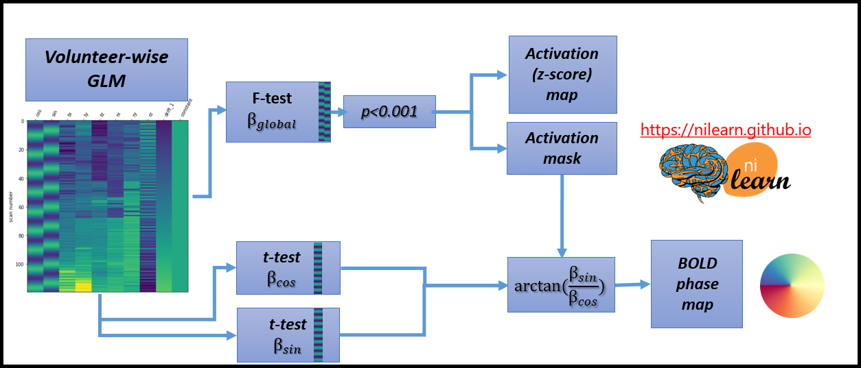
Resting-state data was used to compute the in vivo tSNR. Retinotopic mapping data was analyzed using a subject-wise first-level GLM that included 2 sinusoidal paradigm-related regressors denoted α1 and α2, 6 motion regressors, a drift regressor, and the baseline. The global effect of interest and the BOLD phase maps were estimated as explained in Fig.2.
Results
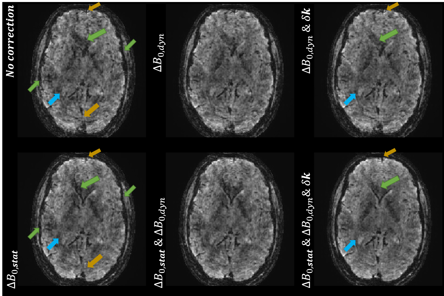
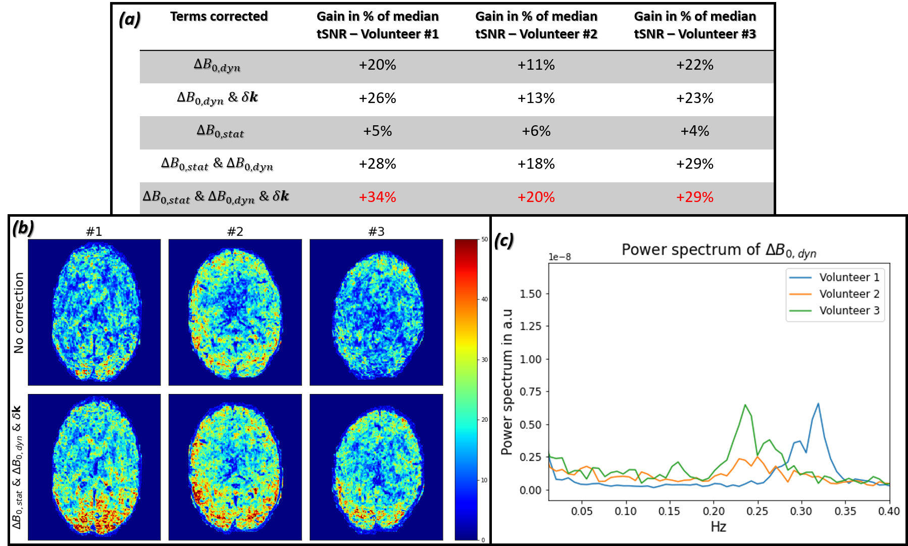
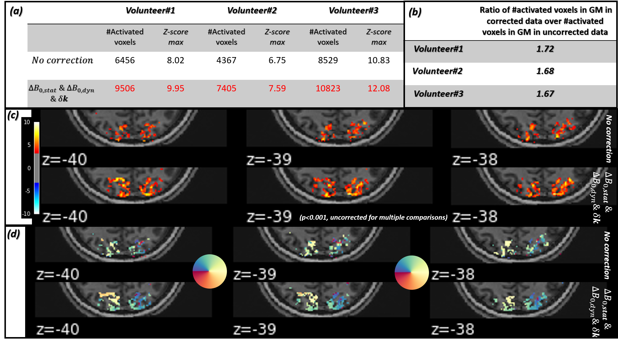
Fig.1-(b) proves that steady state at the level of the probes FID signal is achievable using a TRprobe=50ms and a 470mT*ms/m spoiling gradient. Fig.3 demonstrates the gain in image quality on corrected rs-fMRI data. Fig.4-(a) and (b) illustrate the tSNR improvement: We observed up to 34% gain in median tSNR when correcting the static contribution and up to the first-order dynamic terms. A significant improvement is observed in the visual cortex. Fig.4-(c) shows the power spectrum of the $$$\Delta\textrm{}B_{0,dyn}$$$ term monitored during rs-fMRI for the 3 volunteers. The tables in Fig.5-(a) and (b) report a higher number of activated voxels as well as a higher significance (z-score max) on corrected task-based fMRI data. Fig.5-(c) shows improved and more significant activation maps when correcting field imperfections. Likewise, the BOLD phase maps in Fig.5-(d) are more consistent with the color-gradient of the projection of the retina onto the visual cortex. This is mostly visible for z=-40: The transition from green to orange is more accurate when correcting field imperfections.Discussion
Assuming that resting-state and task-based fMRI images are cleaned similarly when correcting $$$\Delta\textrm{}B_{0}$$$ imperfections, the gain in tSNR observed in Fig.4-(a) and (b) translates into a higher sensitivity to BOLD effect as supported by Fig.5-(a) and (b). In Fig.5-(c), we can observe the emergence of some activations in white matter when correcting field imperfections (z=-40), yet, Fig.5-(b) proves that the sensitivity to BOLD effect is significantly increased in gray matter and the better image quality of the corrected data observed in Fig.3 suggests an improved effective spatial resolution. The BOLD phase maps are also of a higher quality after field imperfections correction.Conclusions
The Skope Clip-on Camera can be used with a short TRprobe if an external spoiling gradient is applied. Furthermore, the highly significant benefit we demonstrated on 3D-SPARKLING fMRI image quality, tSNR and BOLD sensitivity proves that the expected SNR loss in the probes FID signal due to the shorter TR does not degrade the accuracy of the estimated field fluctuations.Acknowledgements
Leducq Foundation (Large Equipement ERPT program, NEUROVASC7T project) provided financial support for this work. Chaithya G.R. was supported by the CEA NUMERICS program, which has received funding from the European Union’s Horizon 2020 research and innovation program under the Marie Sklodowska-Curie grant agreement No 800945. We thank Alexis Amadon for his code for ∆B0 map computation.References
1Chaithya, G.R., Weiss, P., Massire, A., Vignaud, A., Ciuciu, P.: Optimizing full 3D SPARKLING trajectories for high-resolution Magnetic Resonance Imaging. IEEE Transactions on Medical Imaging 41(8), 2105–2117 (2022).
2Amor, Z., Chaithya, G.R., Daval-Frérot, G., Thirion, B., Mauconduit, F.,Ciuciu, P., Vignaud, A.: Prospects of non-Cartesian 3D-sparkling encoding for functional MRI: A preliminary case study for retinotopic mapping. Proceedings of the 30’th Scientific Meeting of the International Society for Magnetic Resonance in Medicine (2022).
3Doneva, M.: Mathematical Models for Magnetic Resonance Imaging Reconstruction. IEEE Signal Processing Magazine 37(1), 24–32 (2020).
4De Zanche, N., Barmet, C., Nordmeyer-Massner, J.A., Pruessmann, K.P.: NMR Probes for Measuring Magnetic Fields and Field Dynamics in MR Systems. Magnetic Resonance in Medecine 60(1), 176–186 (2008).
5Barmet, C., De Zanche, N., Pruessmann, K.P.: Spatiotemporal Magnetic Field Monitoring for MR. Magnetic Resonance in Medecine 60(1), 187–197 (2008).
6Vannesjo, S.J., Wilm, B.J., Duerst, Y., Gross, S., Brunner, D.O., Dietrich,B.E., Schmid, T., Barmet, C., Pruessmann, K.P.: Retrospective Correction of Physiological Field Fluctuations in High-field Brain MRI using Concurrent Field Monitoring. Magnetic Resonance in Medecine 73(5), 1833–1843 (2015).
7Bollmann, S., Kasper, L., Vannesjo, S.J., Diaconescu, A.O., Dietrich, B.E.,Gross, S., Stephan, K.E., Pruessmann, K.P.: Analysis and Correction of Field Fluctuations in fMRI Data Using Field Monitoring. NeuroImage 154(1),92–105 (2017).
8Schwarz, J.M., Stirnberg, R., Ehses, P., Stocker, T.: Correction of Physiological Field Fluctuations in High- and Low-resolution 3D-EPI Acquisitions at 7 Tesla. Proceedings of the 27th Scientific Meeting of the International Society for Magnetic Resonance in Medicine (2019).
9Amor, Z., Chaithya, G.R., Le Ster, C., Daval-Frérot, G., Boulant, N.,Mauconduit, F., Mirkes, C., Ciuciu, P., Vignaud, A.: B0 field distortions monitoring and correction for 3D non-Cartesian fMRI acquisitions using a field camera: Application to 3D-SPARKLING at 7T. Proceedings of the 30’th Scientific Meeting of the International Society for Magnetic Resonance in Medicine (2022)
10El Gueddari, L., Lazarus, C., Carrié, H., Vignaud, A., Ciuciu, P.: Self-calibrating nonlinear reconstruction algorithms for variable density sampling and parallel reception MRI. IEEE 10th Sensor Array and Multichannel Signal Processing Workshop (SAM) (2018).
11Farrens, S., Grigis, A., El Gueddari, L., Ramzi, Z., Chaithya, G.R.,Starck, S., Sarthou, B., Cherkaoui, H., Ciuciu, P., Starck, J.-L.: Pysap:Python sparse data analysis package for multidisciplinary image processing. Astronomy and Computing 32 (2020).
12https://github.com/hbp-brain-charting/public_protocols
13https://github.com/CEA_COSMIC/pysap-mri
14https://www.fil.ion.ucl.ac.uk/spm/doc/biblio/
Figures