2538

Synthesis of Respiratory Phase from Image Phase in Resting-State Functional Magnetic Resonance Imaging

Alexander Jaffray¹, Michelle Medina¹, Christian Kames¹, and Alexander Rauscher^1,2
¹Physics, UBC MRI Research Centre, Vancouver, BC, Canada, ²Department of Pediatrics, UBC, Vancouver, BC, Canada

Synopsis

Keywords: Data Processing, fMRI (resting state), Breathing Belt, Respiratory Phase

Functional Magnetic Resonance Imaging (fMRI) is routinely acquired using gradient-echo sequences with long echo times and short repetition time. Such sequences encode information about the magnetic field in the often discarded image phase. We demonstrate a method for processing the phase of reconstructed fMRI data to isolate temporal fluctuations in the harmonic fields associated with respiration by solving a blind source separation problem. Computed respiratory phase from the fMRI-derived field fluctuations was shown to be in strong agreement with breathing belt data acquired during the same scan. This work thus presents a hardware free measurement of respiratory phase.

Introduction

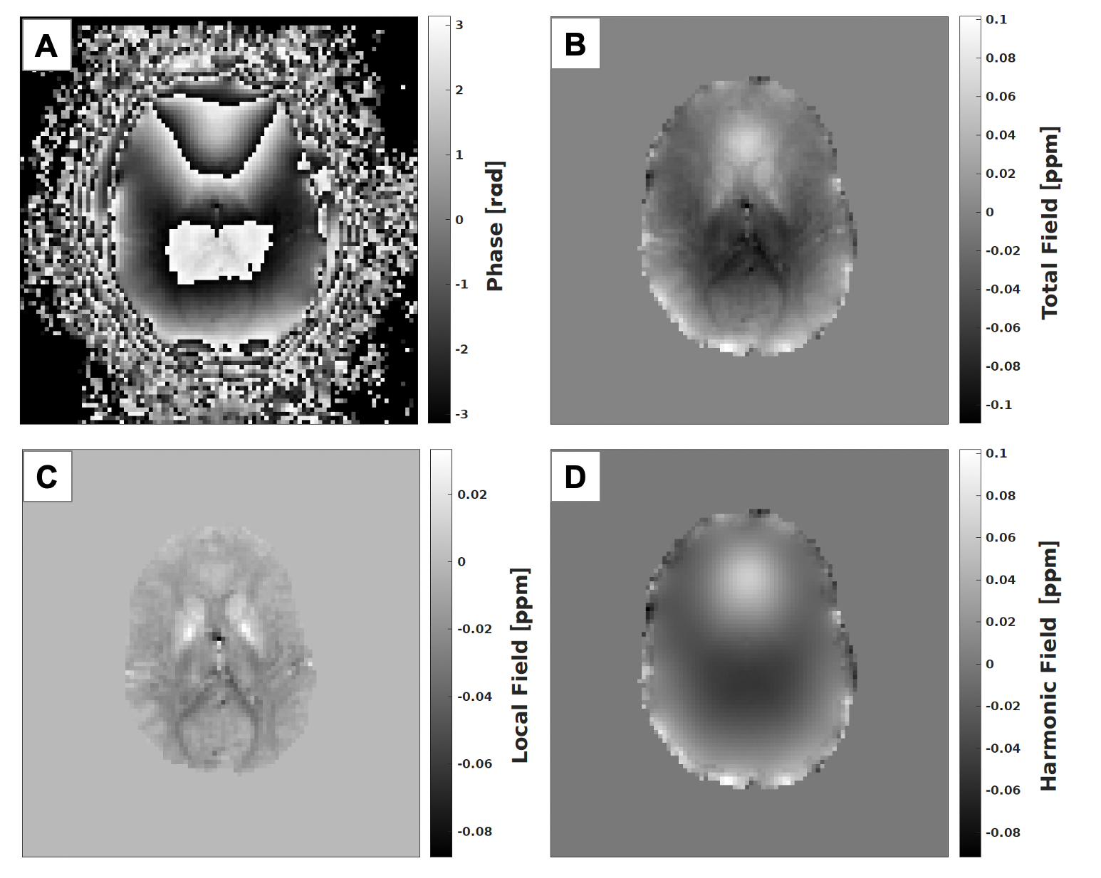
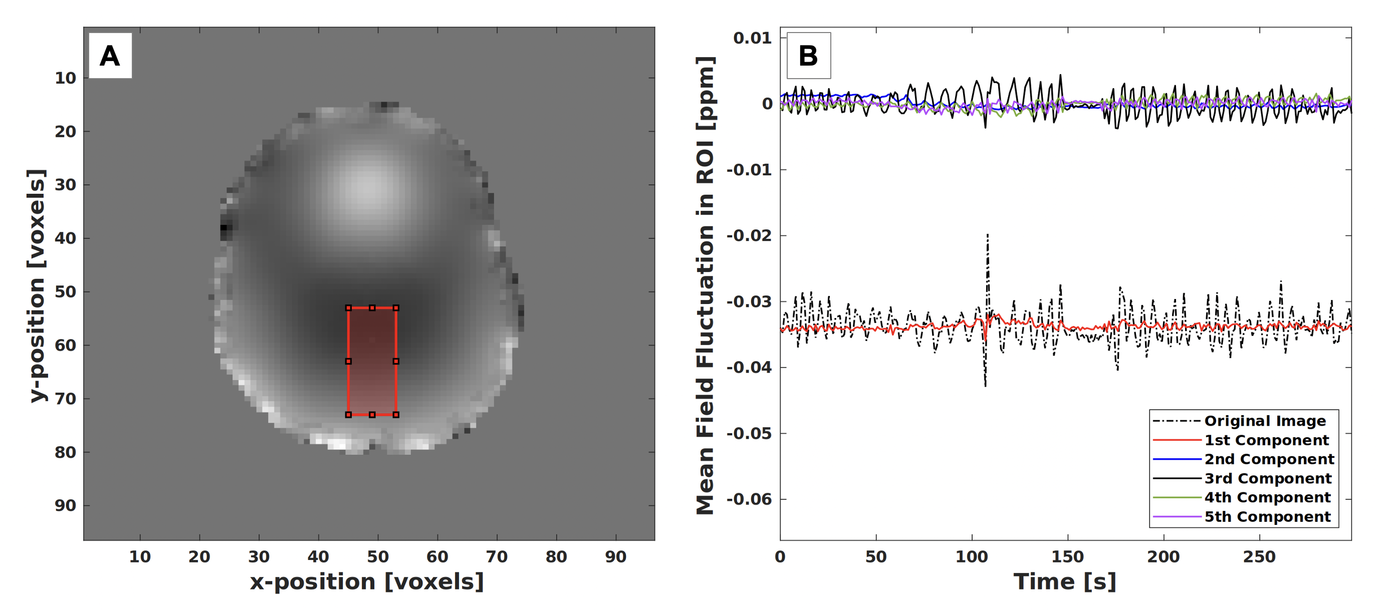
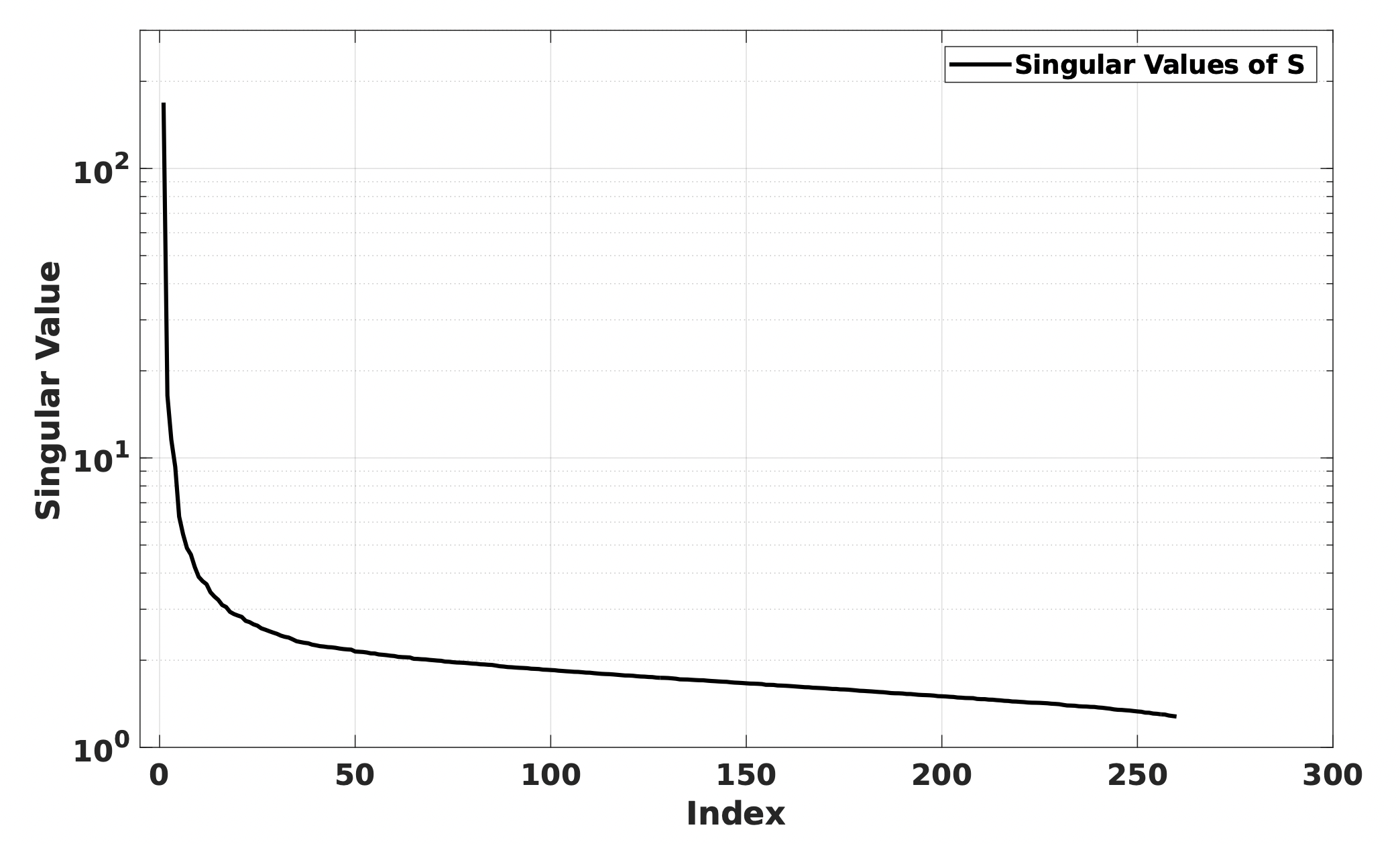
Acquisition of functional magnetic resonance (fMRI) images commonly utilizes single-shot gradient echo (GRE) echo-planar imaging (EPI) sequences, enabling acquisition at high temporal resolutions.^1,2 GRE sequences are also widely used to acquire phase images which are processed using techniques including Quantitative Susceptibility Mapping (QSM) and Susceptibility Weighted Imaging (SWI).^3-7 Each reconstructed fMRI volume is a complex-valued depiction of the magnitude and phase of the magnetization sampled at the echo time (TE). It has been shown that respiration induces fluctuations in the magnetic field inside the brain of between 2-5 Hz, contributing to physiological noise in the fMRI measurement.^8,9 Data-driven corrections to the fMRI signal are possible but can mistake signal for physiological noise, thus external monitoring is usually used to correct physiological noise.¹⁰ Image phase, commonly ignored in fMRI, is sensitive to breathing-induced fluctuations in the magnetic field. This range of of fluctuation is also within the sensitivity range of QSM processing routines.⁴ Background field estimation and subtraction is a necessary step in QSM to separate global (harmonic) magnetic field changes and susceptibility-induced changes in the local magnetic field arising within the imaging volume.¹¹ Harmonic fields are not usually explicitly computed for QSM but can be obtained by subtracting the estimated tissue field from the total field.

We propose to process the phase of whole-brain resting-state fMRI sequences with short TR to capture respiration-induced changes in the harmonic field within the imaging volume. The time-course of the harmonic field is decomposed via SVD to separate breathing-induced field modulations from other sources of noise.¹² The resulting field modulation trace can then be used to estimate the respiratory phase during acquisition in a robust manner.

Methods

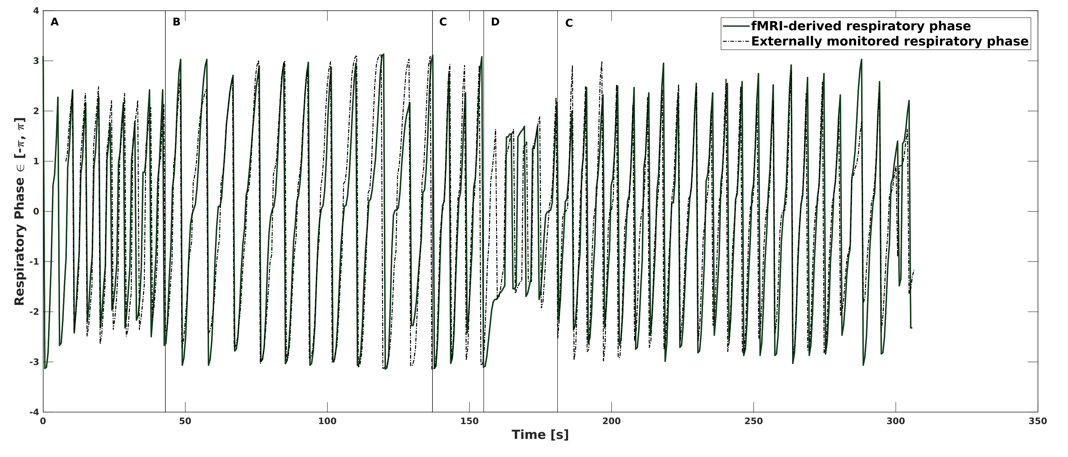
We performed a single volunteer study, acquiring a resting-state fMRI scan at 3T (Philips Elition) of approximately 5 minutes in duration using a gradient-echo EPI sequence with a SENSE factor of 4 and TR/TE of 1150/30. An isotropic voxel size of 2.5 mm and multi-band factor of 2 was employed. Complex data was reconstructed and exported at the console. The size of the reconstructed data was 96x96x57x260 corresponding to 3 spatial dimensions and a temporal dimension.

Respiration of the subject was monitored using the scanner's respiratory physiology sensor. The subject was instructed to perform a series of controlled breathing patterns during the scan:

10 short breaths
10 deep breaths
free-breathing
breath-hold (10-20s)
free-breathing

After acquisition, the resting-state fMRI data was sliced along the temporal dimension to produce 260 volumes which were processed (Fig. 1) using the following steps:

Laplacian-based phase unwrapping¹³
Local field estimation with regularized SHARP¹¹
Harmonic field estimation

The estimated harmonic field data was reshaped into a $$$M \times N$$$ matrix $$$\mathbf{P}$$$ where $$$M$$$ is the number of spatial voxels and $$$N$$$ is the number of time samples during the acquisition. P was then decomposed using Singular-Value Decomposition (SVD) and a temporally low-rank representation of the background field $$$\mathbf{P}_L$$$ was reconstructed by truncating the diagonal of the matrix $$$\mathbf{S}$$$ to obtain $$$\mathbf{S}_L$$$.¹⁴ $$\mathbf{P} = \mathbf{U}\mathbf{S}\mathbf{V}^T$$ $$\mathbf{P}_L = \mathbf{U}\mathbf{S}_L\mathbf{V}^T$$The time-course of the coefficients of the first 5 eigenvectors $$$p_i(t): i \in [1,5]$$$ of the low-rank representation was subsequently calculated (Fig. 2). Discrimination of the $$$p_B(t)$$$ corresponding to breathing was performed by finding the coefficient with the maximal instantaneous temporal variation, accomplished by choosing the $$$p_i(t)$$$ which maximized $$$\lVert \frac{dp_i(t)}{dt}\rVert_1$$$. Processing of the data was performed in MATLAB and took ~150s on a 32-core workstation.

Synthesis of respiratory phase was performed using the method proposed for RETROICOR, and applied to both $$$p_B(t)$$$ and the respiratory sensor signal $$$R(t)$$$ after upsampling $$$p_B(t)$$$ by a factor of 2 and resampling to a common dwell time.¹⁵ Phase-derived and reference respiratory phase were compared.

Results

Synthesized respiratory phase agreed strongly with respiratory phase obtained from the breathing belt (Fig. 4). Distinct periods of controlled breathing were seen in both synthesized and reference traces corresponding directly with subject instruction. Mean-square error in the measured respiratory period was 0.3s. The spectrum of singular values (Fig. 3) obtained from the SVD of $$$\mathbf{P}$$$ was consistent with the assumption that fluctuations in the harmonic field were low-rank in the temporal dimension.

Correspondence with the reference respiratory phase was maintained across shallow, deep and free-breathing periods. The breath-hold period shows similar, erratic behaviour across both traces, which can be attributed to limited filtering of the obtained traces.

Discussion

We demonstrate the feasibility of hardware-free synthesis of respiratory phase from resting-state fMRI image phase that is robust to scan acceleration and independent of the fMRI experiment. The method can be applied retrospectively if the image phase is available, and facilitates improved physiological noise correction in fMRI studies for which external physiology monitoring is not available.

A limitation is that TR must be shorter than half of the shortest respiration period, a necessary condition for respiratory trace reconstruction. Fortunately, there is significant effort in fMRI research to increase temporal resolution with novel image acquisition and reconstruction strategies.^16-18

Future work will validate our technique on a large cohort of participants in a concussion study currently ongoing at the UBC MRI Research Centre. Implementations of the phase processing algorithms used in this work are part of the open-source QSM toolbox from Christian Kames.¹⁹

Acknowledgements

All work was conducted at the University of British Columbia, located on the traditional, ancestral and unceded territory of the Musqueam people.

References

1. Glover GH. Overview of Functional Magnetic Resonance Imaging. Neurosurg Clin N Am 2011;22:133–139 doi: 10.1016/j.nec.2010.11.001.

2. Ogawa S, Tank DW, Menon R, et al. Intrinsic signal changes accompanying sensory stimulation: functional brain mapping with magnetic resonance imaging. Proc. Natl. Acad. Sci. U.S.A. 1992;89:5951–5955 doi: 10.1073/pnas.89.13.5951.

3. Wang Y, Liu T. Quantitative susceptibility mapping (QSM): Decoding MRI data for a tissue magnetic biomarker. Magnetic Resonance in Medicine 2015;73:82–101 doi: 10.1002/mrm.25358.

4. Deistung A, Schweser F, Reichenbach JR. Overview of quantitative susceptibility mapping: Overview of Quantitative Susceptibility Mapping. NMR Biomed. 2017;30:e3569 doi: 10.1002/nbm.3569.

5. Reichenbach JR, Haacke EM. Gradient Echo Imaging. In: Susceptibility Weighted Imaging in MRI. John Wiley & Sons, Ltd; 2011. pp. 33–46. doi: 10.1002/9780470905203.ch3.

6. Reichenbach JR, Venkatesan R, Schillinger DJ, Kido DK, Haacke EM. Small vessels in the human brain: MR venography with deoxyhemoglobin as an intrinsic contrast agent. Radiology 1997;204:272–277 doi: 10.1148/radiology.204.1.9205259.

7. Rauscher A, Sedlacik J, Deistung A, Mentzel H-J, Reichenbach JR. Susceptibility Weighted Imaging: Data Acquisition, Image Reconstruction and Clinical Applications. Zeitschrift für Medizinische Physik 2006;16:240–250 doi: 10.1078/0939-3889-00322.

8. Van de Moortele P-F, Pfeuffer J, Glover GH, Ugurbil K, Hu X. Respiration-induced B0 fluctuations and their spatial distribution in the human brain at 7 Tesla. Magnetic Resonance in Medicine 2002;47:888–895 doi: 10.1002/mrm.10145.

9. Vannesjo SJ, Miller KL, Clare S, Tracey I. Spatiotemporal characterization of breathing-induced B0 field fluctuations in the cervical spinal cord at 7T. NeuroImage 2018;167:191–202 doi: 10.1016/j.neuroimage.2017.11.031.

10. Bulte D, Wartolowska K. Monitoring cardiac and respiratory physiology during FMRI. NeuroImage 2017;154:81–91 doi: 10.1016/j.neuroimage.2016.12.001.

11. Sun H, Wilman AH. Background field removal using spherical mean value filtering and Tikhonov regularization. Magnetic Resonance in Medicine 2014;71:1151–1157 doi: 10.1002/mrm.24765.

12. Golub GH, Reinsch C. Singular value decomposition and least squares solutions. Numer. Math. 1970;14:403–420 doi: 10.1007/BF02163027.

13. Schofield MA, Zhu Y. Fast phase unwrapping algorithm for interferometric applications. Opt. Lett., OL 2003;28:1194–1196 doi: 10.1364/OL.28.001194.

14. Wold S, Esbensen K, Geladi P. Principal component analysis. Chemometrics and Intelligent Laboratory Systems 1987;2:37–52 doi:10.1016/0169-7439(87)80084-9.

15. Glover GH, Li TQ, Ress D. Image-based method for retrospective correction of physiological motion effects in fMRI: RETROICOR. Magn Reson Med 2000;44:162–167 doi: 10.1002/1522-2594

16. Moeller S, Yacoub E, Olman CA, et al. Multiband multislice GE-EPI at 7 tesla, with 16-fold acceleration using partial parallel imaging with application to high spatial and temporal whole-brain fMRI. Magnetic resonance in medicine 2010;63:1144–1153.

17. Kasper L, Engel M, Heinzle J, et al. Advances in spiral fMRI: A high-resolution study with single-shot acquisition. NeuroImage 2022;246:118738 doi: 10.1016/j.neuroimage.2021.118738.

18. Engel M, Kasper L, Patzig F, Bianchi S, Prüssmann, K. Whole-brain fMRI at 5 frames per second using T-Hex spiral acquisition. Proceedings of the International Society for Magnetic Resonance in Medicine (ISMRM) 2021; Abstract 0886.

19. Kames C, Wiggermann V, Rauscher A. Rapid two-step dipole inversion for susceptibility mapping with sparsity priors. Neuroimage 2018;167:276–283 doi: 10.1016/j.neuroimage.2017.11.018.

Figures

Figure 1. Processing Pipeline from Image Phase to Background Field: A) Image phase obtained after scanner reconstruction. B) Total field estimate after Laplacian-based unwrapping, containing global and local field contributions.¹³ C) Local field estimate after harmonic field removal using ReSHARP algorithm.¹¹ D) Estimated background field in parts per million of the main magnetic field.

Figure 2. Decomposition of Background Field Fluctuations: A) Background field estimate of a sample slice. The red rectangular selection indicates a region of interest over which temporal field fluctuations are estimated. B) Time dependent fluctuations of the background field within the selected region of interest, and the temporal evolution of the coefficients of the first 5 eigenvectors found in the decomposition of $$$\mathbf{P}$$$ using the SVD.

Figure 3. Singular Value Decomposition: Singular values of the matrix $$$\mathbf{S}$$$ arranged from largest to smallest resulting from the decomposition of $$$\mathbf{P}$$$. A steep gradient is observed in the magnitude after the first few singular values, consistent with the hypothesis that $$$\mathbf{P}$$$ can be approximated well by the low-rank matrix $$$\mathbf{P}_L$$$.

Figure 4. Comparison of fMRI-derived and reference respiratory traces: The solid line shows the respiratory trace calculated from the fMRI image phase, and the dashed line shows the reference respiratory trace computed from the external physiology sensor. Excellent agreement between the traces is shown, with mean-square error in respiratory period of 0.3 s. The periods of structured breathing are indicated as follows: A) Shallow breathing B) Deep breathing C) Free breathing D) Breath hold

Proc. Intl. Soc. Mag. Reson. Med. 31 (2023)

2538

DOI: https://doi.org/10.58530/2023/2538