2420
Longitudinal Modeling of Stroke using Stochastic Distances and NODDI Diffusion Model1Radiology and Imaging Sciences, University of Utah, Salt Lake City, UT, United States
Synopsis
Keywords: Data Analysis, Machine Learning/Artificial Intelligence, Stroke diffusion modeling
Limited prior work has explored longitudinal modeling of human brain stroke using advanced diffusion techniques. We aim to address this gap by analyzing longitudinal stroke data from diffusion spectrum imaging for modeling and predicting clinical markers of stroke recovery. Our proposed data analysis method uses a mixed-effect model which exploits stochastic distances from these images for improved regression model statistics and handling of imbalanced, inconsistent longitudinal data. We also demonstrate that this aids in differentiating between population-level and patient-level effects and the corresponding key contributing predictors at each of these levels.Introduction
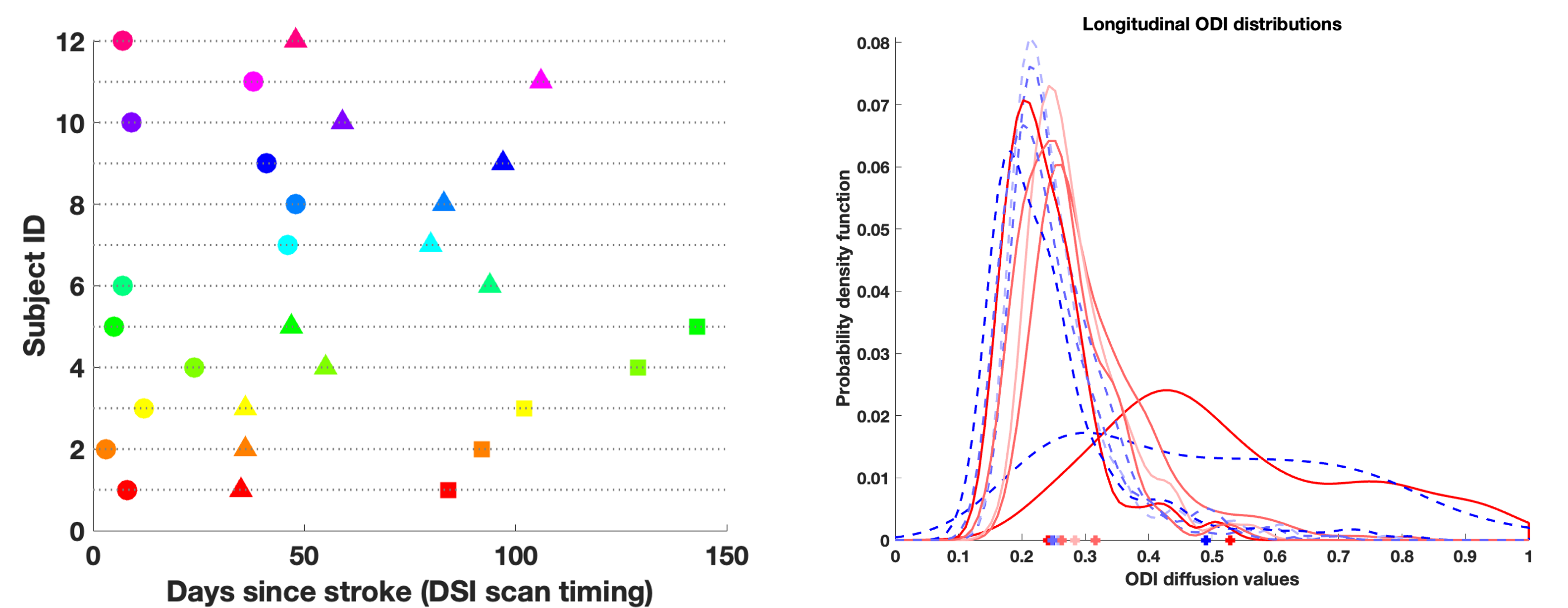
Diffusion MRI has been a widely used to study brain stroke. While most studies use DTI1, recent studies have focused on advanced diffusion techniques (e.g. DKI2, NODDI3 which incorporate sophisticated biophysical modeling and have shown improvements over DTI in post-stroke analysis and recovery predictions4. However, most of these use a single timepoint in the acute phase (< 1 month of stroke)4. Very few studies analyze both acute and chronic stages5,6,7 and use a group-wise comparison strategy which doesn’t fully exploit the repeated-measure design. In contrast, we present our analysis on Diffusion Spectrum Imaging (DSI) data acquired longitudinally for each stroke subject to model clinical markers of stroke recovery. We hope to characterize immediate as well as long-term post-stroke biophysical changes leading to an improved understanding of stroke recovery and subsequent therapy choices.Our planned timings for MRI acquisitions are ~2 weeks, 1 month and 3 months. However, despite an initially well-thought study design, often practical limitations arise due to patient unavailability. For example, Fig. 1 (left) shows that longitudinal MRI scans for most patients do not align with these planned timings, including several missing scans. This makes a group-wise analysis inaccurate due to large intra-group variability. We propose using a mixed-effect model which can successfully handle imbalanced and missing timepoints and benefits from a joint estimation of the overall population trend as well as patient-specific trends. However, instead of conventional mixed-effect modeling, we show that whenever possible, using stochastic ‘distances’ inside these models leads to improved model statistics (Fig.1 (right)). Prior work has shown that stochastic ‘distance’ measures can be used to quantify the dissimilarity between two image regions-of-interest (ROI). They are more powerful in their ability to capture ROI differences than the traditional approach of using the ‘mean diffusion value’ as the ROI summary8,9,10,11.
Method
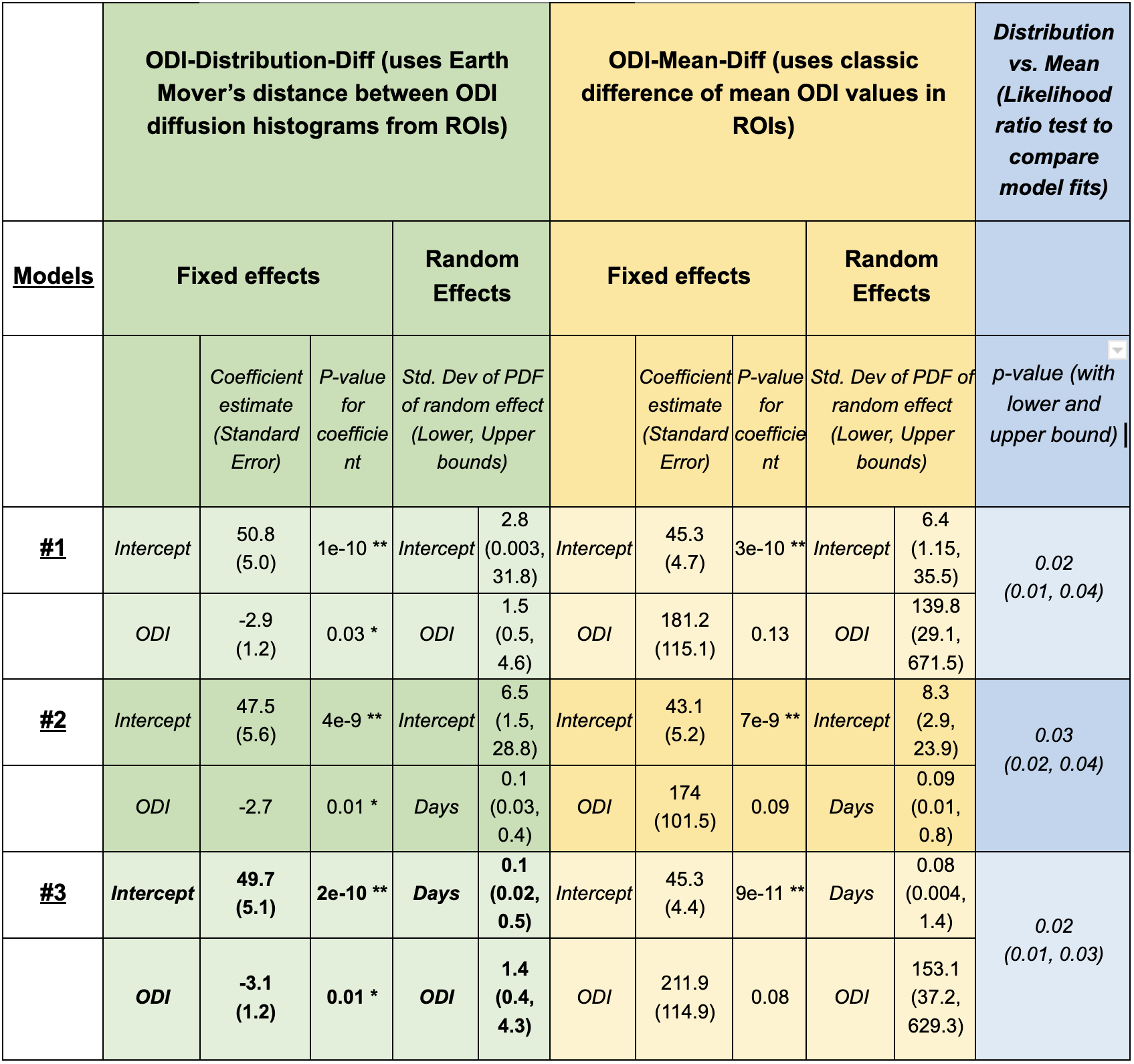
Longitudinal DSI data is acquired from 12 stroke subjects: 5 with 3 timepoints, 7 with 2 timepoints (Fig.1, 3T scanner, NODDI model based on DSI, 203 directions, max b=4000). Corresponding clinical scores (Fugl-Meyer) indicating recovery are also acquired. We use the ODI diffusion values (Orientation dispersion index from the NODDI model3) from the motor tract as they are an important biomarker of post-stroke recovery12. The mixed-effect regression model uses the following: longitudinal clinical scores (response variable), subject ID (grouping variable), number of ‘days’ since stroke to capture the DSI scan timings (predictor variable 1), inter-hemispheric difference in the ODI values from the motor ROI (predictor variable 2).The inter-hemispheric ODI differences are captured in one of two ways. 1) ‘ODI-Mean-Diff: ROI represented via mean ODI value, with difference as {Mean ODI (Ipsilateral) - Mean ODI (Contralateral)}. 2) ODI-Distribution-Diff (ROI represented using the entire histogram of ODI values, with difference as the Earth Mover Distance between Ipsilateral and Contralateral ODI histograms11,10. After systematically exploring various model choices and variable combinations using likelihood-ratio tests, we summarize the findings from the top three models in Fig. 2 (based on statistical significance of fixed and random regression coefficients and model comparison tests, low standard errors, tight lower-upper bounds). For each model choice, the fixed effect is the overall population-level trend and the random effect is the patient-level deviation from the fixed effect. Both fixed and random effects may include intercept, any of the predictor variables and their combinations.
Results
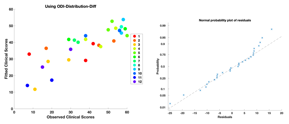
Longitudinal ODI values are an important predictor at the population-level (along with the intercept) (Models 1,2,3 in Fig. 2, Fig. 3). This matches prior work where diffusion imaging can help with clinical recovery prediction1,4. Individual variability in ODI values is also important to subject-specific trends (Models 1,3). Additionally, due to subject-specific scan timing inconsistencies, ‘days’ is also a critical predictor for the random-effects (Models 2,3).Results also demonstrate that any model using ‘ODI-Mean-Diff' distances, fails to find a statistically significant, population-level ODI trend. Even though the intercept is significant, it does not inform about the value of any of the predictor variables. In contrast, when we use ‘ODI-Distribution-Diff' distances, all models find statistically significant, population ODI trend. Note that a lower-upper bound for the random effect which doesn’t include zero, indicates a significant subject-specific deviation from the population’s fixed effect. Since all models have these bounds outside zero, this points to the importance of mixed-effects modeling which can differentiate the underlying subject-specific effects from the overarching fixed-effects while also identifying the corresponding key contributing predictors for each of these effects.
A likelihood ratio test to compare the ‘ODI-Mean-Diff' models with ‘ODI-Distribution-Diff' (last column, Fig. 2) further highlights that stochastic-distances provide better model fits than mean-distances. Overall, Model 3 using ‘ODI-Distribution-Diff', gives the best results, with Model 2 with ‘ODI-Distribution-Diff', being a close second.
Conclusion
We demonstrate the value of longitudinal modeling for stroke using advanced diffusion techniques. The results are promising and must be validated further on larger datasets. By using data efficiently and jointly across subjects (versus individual patient modeling or dummy variables per subject), a mixed-effect longitudinal model scales better to larger datasets and naturally accounts for correlation in repeated scans. Stochastic ‘distance’ measures when plugged into classic mixed-effect settings, create an easy but powerful method to exploit subtle, nuanced differences hidden within image ROIs.Acknowledgements
We are grateful to Dr. Jennifer Majersik, Dr. Lorie Richards, Kinga Aitken, and Dr. Ganesh Adluru of the University of Utah for assisting with the stroke dataset used for this study.References
1. Moura, L. M., Luccas, R., ... & Conforto, A. B. (2019). Diffusion tensor imaging biomarkers to predict motor outcomes in stroke: a narrative review. Frontiers in neurology, 10, 445.
2. Steven, A. J., Zhuo, J., & Melhem, E. R. (2014). Diffusion kurtosis imaging: an emerging technique for evaluating the microstructural environment of the brain. American journal of roentgenology, 202(1), W26-W33.
3. Zhang, H., Schneider, T., … & Alexander, D. C. (2012). NODDI: practical in vivo neurite orientation dispersion and density imaging of the human brain. Neuroimage, 61(4), 1000-1016.
4. DiBella, E. V. R., Sharma, A., … & Hashemizadeh, S. K. (2022). Beyond diffusion tensor MRI methods for improved characterization of the brain after ischemic stroke: a Review. American Journal of Neuroradiology, 43(5), 661-669.
5. Lampinen, B., Lätt, J., … & Nilsson, M. (2021). Time dependence in diffusion MRI predicts tissue outcome in ischemic stroke patients. Magnetic resonance in medicine, 86(2), 754-764.
6. Mastropietro, A., Rizzo, G., ... & Grimaldi, M. (2019). Microstructural characterization of corticospinal tract in subacute and chronic stroke patients with distal lesions by means of advanced diffusion MRI. Neuroradiology, 61(9), 1033-1045.
7. Granziera, C., Daducci, A., ... & Krueger, G. (2012). A new early and automated MRI-based predictor of motor improvement after stroke. Neurology, 79(1), 39-46.
8. Sharma, A., Fletcher, P. T., ... & Gerig, G. (2013, April). Spatiotemporal modeling of distribution-valued data applied to dti tract evolution in infant neurodevelopment. In 2013 IEEE 10th International Symposium on Biomedical Imaging (pp. 684-687). IEEE.
9. Sharma, A., & Gerig, G. (2020, October). Trajectories from Distribution-Valued Functional Curves: A Unified Wasserstein Framework. In International Conference on Medical Image Computing and Computer-Assisted Intervention (pp. 343-353). Springer, Cham.
10. Sharma, A. (2021). Temporal Modeling and Analysis of Distribution-Valued Functional Curves: Application to Diffusion Tensor Imaging. PhD Dissertation. University of Utah.
11. Peyré, G., & Cuturi, M. (2019). Computational optimal transport: With applications to data science. Foundations and Trends® in Machine Learning, 11(5-6), 355-607.
12. Hodgson, K., Adluru, G., … & DiBella, E. (2019). Predicting motor outcomes in stroke patients using diffusion spectrum MRI microstructural measures. Frontiers in neurology, 10, 72.
Figures