Synopsis

Keywords: Software Tools, Spectroscopy, Data Analysis, Metabolism

Brain tumor metabolic maps are one application of non-invasive MR Spectroscopy (MRS), although there are many other areas of patient treatment and surgery planning that would benefit from improved MRS analysis. A fast, accurate new method for MRS is used here to estimate the ratio of Choline to NAA from simulated spectra modeled on those near a brain tumor, using simple formulas for determining the FID amplitudes that relate to metabolite intensities and concentrations. No approximate numerical integration is required. The time of computation of 0.052 seconds per voxel speeds the construction of a metabolic 3D brain map.

Introduction

High accuracy of metabolite ratios or concentrations is important in many applications of MRS, such as for constructing a 3D map of a brain tumor for surgical intervention^1,2. Requiring analysis of many voxels for resolution, the speed of computation is also critical. Our new method for post-processing MRS data called mdMRS ³ has a number of advantages that apply: (i) removal of baseline offset and phase correction are simple, quick, and effective, (ii) no large basis set of metabolites is required, and (iii) accuracy of FID amplitude, which is proportional to area under the phase-corrected peak profile, is increased with a novel iteration similar to spectral editing, but used here during post-processing. No numerical integration required. Results of an application of this new method for metabolite ratios are shown for simulated but realistic data, with emphasis on the Choline/NAA ratio.

Methods

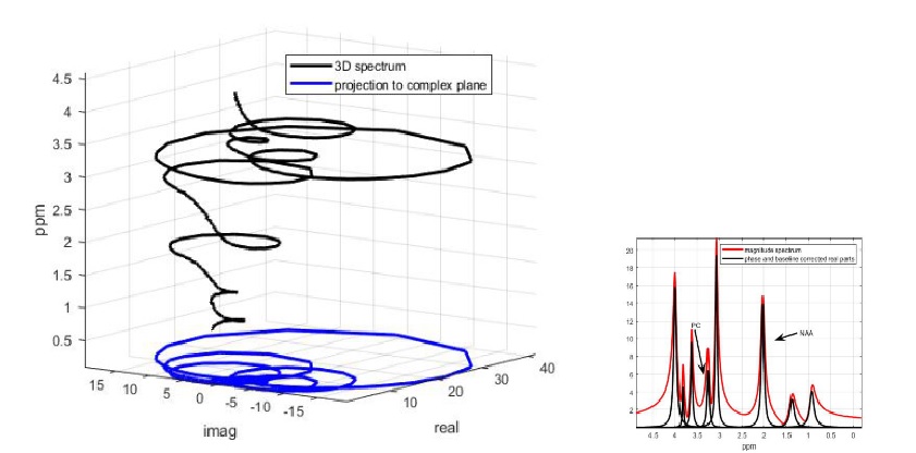
The FID data from the MR scanner is assumed to be a sum of terms of the form $$$\text{FID}(t) = A e^{-t/T_2^*}e^{i\phi}e^{2\pi i\nu t},$$$ where $$$A, T_2^*, \phi, \nu$$$ are the amplitude, damping constant, phase angle and frequency location. $$$\ \ $$$ Importantly, A is proportional to ``spectral peak area^''4. The FID has continuous Fourier transform (cFT) that is found by applying the integral formula for the cFT with the assumption that the FID(t) is zero for $$$t<0.$$$ The cFT transform is given by $$cFT_\mathrm{{FID}} (w) = \frac{A e^{i \phi}}{1/T_2^* +2\pi i (w-\nu)} = \frac{b-a d}{w+d}, $$ where constants $$$a = 0, b = A e^{i \phi}/(2\pi i), $$$ and $$$d= 1/(2\pi i T_2^*) - \nu$$$ are included in this form partly to emphasize that the only variable for the cFT transform of the FID is the frequency variable $$$w.$$$ It is not difficult to use the above equation to show that the transform, $$$cFT_{\mathrm{FID}}(w)$$$ is the equation of a circle in the complex plane. This feature was known and used in novel software called CFIT⁵. Based on the form of the transform as a circle, the mdMRS method extends that work to a new 3D-based method for analyzing MRS data, with the prefix md emphasizing the goal of making the results useful to medical doctors..

It is natural to do MRS analysis in 3D, since the FID transform is inherently three-dimensional. The DFT of an FID is 2D, (real(DFT), imag(DFT), and frequency is the third dimension. See Figure 1. Only three valid points on a peak profile are needed to construct that profile completely, since three points determine a circle. Further this is also true for the cFT of the FID. The rightmost term in the displayed formula above is a Linear Fractional Transform(LFT), that is a well-studied form which has many known properties. The connection to an LFT results in a simple formula for the amplitude A given by $$$A = 2\pi |ad-b|$$$ which is proportional to the area used for MRS analysis. This mdMRS formula for A is both simple and easy to compute, as well as being very accurate.

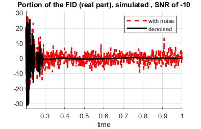
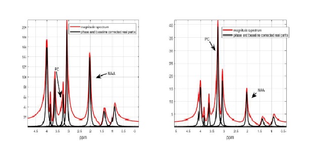
Simulated data based on patient data consisting of eight peak profiles was analyzed with additive white gaussian noise at three different noise levels. Denoising was applied to the noisy FID using wavelet denoising and then a Tukey filter. Figure 2 shows the noisy(red) and denoised(black) FID. See Figure 3 for the magnitude spectrum for the two ratio cases considered: low and high Choline/NAA ratio. The new mdMRS methods, including the iterative refinement of amplitude estimates method that is similar to spectral editing but done in post-processing, was applied to obtain the best estimates of FID amplitudes.

Results.

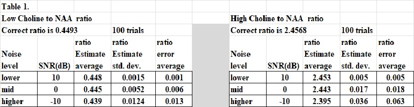
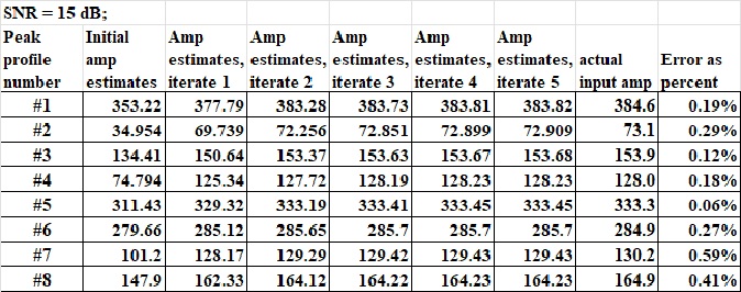
The amplitude estimates for both the low Choline/NAA ratio (0.449) and high ratio (2.457) show excellent results as listed in Table 1. The three noise levels considered go from lower (10dB), mid (0dB), to higher ($$$-$$$10 dB). For the low Choline/NAA ratio value and for the lower noise level, the average error was only 0.001, or about 0.3% relative error. Not listed is that this high accuracy is achieved for all lower noise levels as well. At the mid or higher noise levels, the accuracy decreases somewhat, but even at the highest noise level considered the average error had the low value of 2.9% relative error. For the high ratio value with Choline more than NAA (as for a brain tumor voxel), the relative amplitude errors were 0.2%, 0.7%, and 2.9% for the three different noise levels.

The new iterative mdMRS sharpening method, similar to spectral editing, provided nearly perfect convergence to the correct input amplitudes for FID with lower noise levels (SNR of 15dB or more), as shown in Table 2. Those results show that any ratio of two of the eight amplitude estimates will be nearly perfect in this case, and not just the Choline/NAA ratio The noisier FID input cases are not shown in Table 2, but again have small relative errors. .

Conclusion.

The time of computation for analysis of one spectrum is about 0.052 seconds on a PC with Intel i7 running at 2.8 GHz using MATLAB. This speed would reduce the analysis time of the large number of spectra needed for brain tumor localization in 3D.

Acknowledgements

The author wishes to thank William S. Clary, Ph.D., mathematician, most recently of the University of Akron, for technical conversations and ideas. Thanks also to D. Jenkins, M.D., neonatologist at MUSC for many helpful remarks and suggestions. In addition, thanks to Hunter W. Moss, Ph.D. for assistance with data handling.