Synopsis

Keywords: Software Tools, Motion Correction, motion simulation

To investigate the possibility and limitation of MRI simulations based on the Lagrange description, MRI experiments and simulations of moving objects were performed. As a result, we were able to obtain simulated MR images that almost reproduced the experimental results within practical computation time. However, it was found that the T2 coherence effect should be reduced for moving objects. It was also found that more precise simulation is necessary to reproduce the detailed motion artifacts.

Introduction

Bloch equations are widely used to numerically reproduce MRI phenomena^1-8. In the Euler description of the Bloch simulation, the nuclear spins are fixed to a coordinate system, while in the Lagrange description, the positions of the nuclear spins are followed throughout the pulse sequence. The Euler description is widely used in quantitative MRI, and the Lagrange description is mainly used in simulation of fluid flow in MRI. In this study, Bloch equations based on the Lagrange description are applied to moving objects to clarify the possibility and limitations of MRI simulations.

Materials and methods

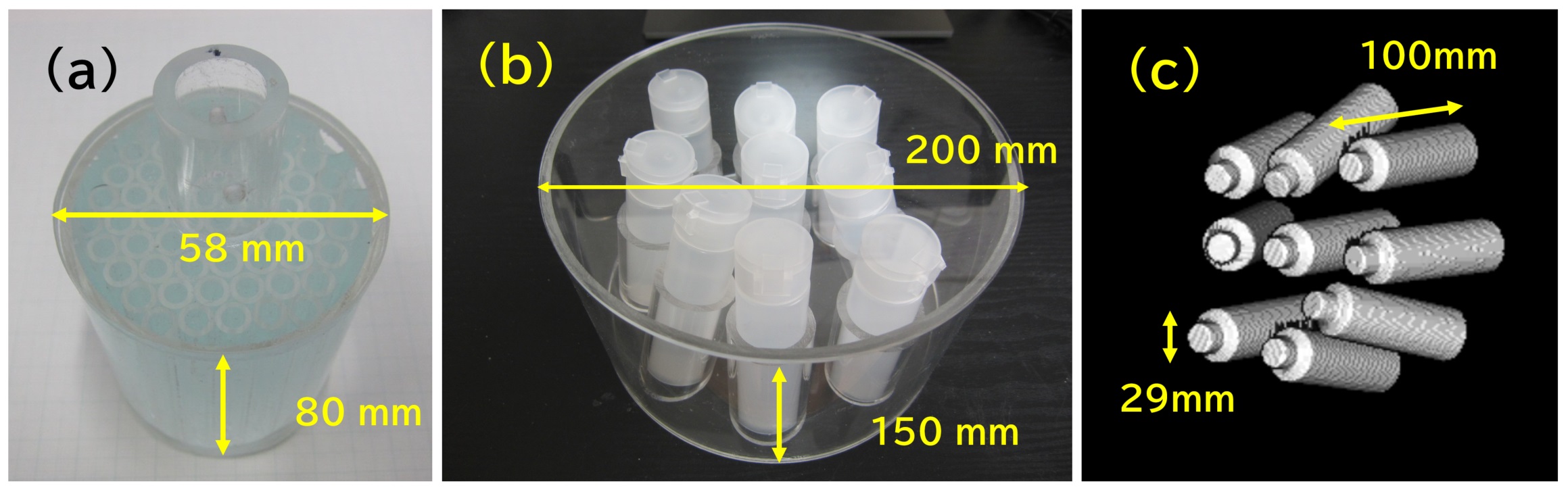
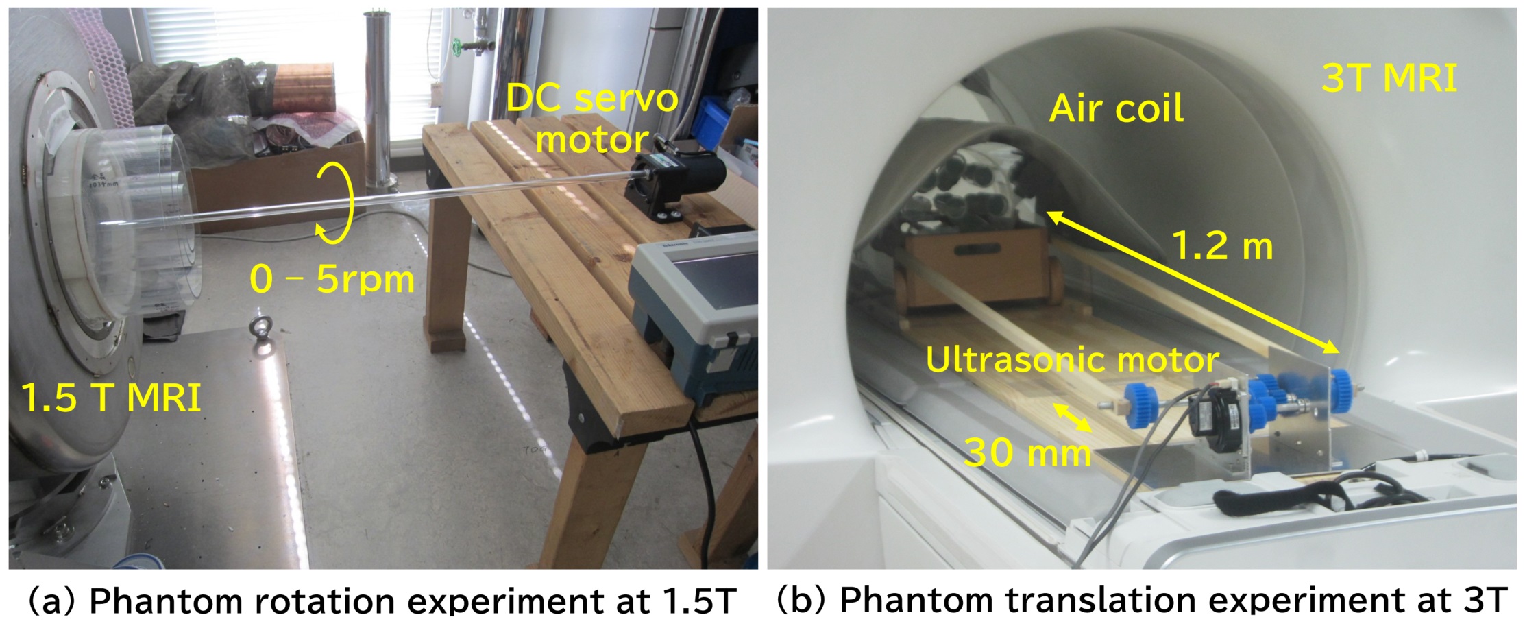
Figure 1 shows the phantoms used in this study. As shown in Fig. 2(a), the rotation experiment was performed by rotating the phantom with a DC servo motor through an acrylic pipe. The MRI system used in the experiment was a digital MRI system with a 1.5 Tesla superconducting magnet with a 280 mm bore. The pulse sequence was a GRE sequence with TR=20ms and TE=8ms. 20 consecutive images were acquired at 3 second time-intervals at a constant rotation speed. As shown in Fig. 2(b), the translation experiments were performed using a driving system consisting of a non-magnetic ultrasonic motor and plastic gears. The water phantom was placed on a wooden dolly and driven with two 1.2 m long wooden cranks connected to the driving system. The amplitude of the translational motion was 30 mm, and the period was 3.8 seconds to simulate respiratory motion. The MRI system used in this experiment was a 3T clinical MRI (SIGNA Premier). The pulse sequences were axial and coronal 2D GRE sequences with TR=4.224ms, TE=2.1ms, and 8mm slice thickness. 40 consecutive images were acquired at 0.54 second time-intervals.
Bloch simulation of the rotation was performed using the Lagrange description, in which the position of the proton rotates at a constant angular velocity, and at each position, the proton receives RF and gradient pulses according to the pulse sequence and simultaneously undergoes nuclear magnetic relaxation. The time increments for the calculation were 20 microseconds, and the Bloch equations were solved numerically at each time increment to calculate the MR signal. The number of spins used for the calculation was 65,536 and the total number of the time steps for one image was 138,000. Bloch simulation of the translational motion was performed by the Lagrange description, in which the numerical phantom moved sinusoidally in the horizontal plane along the z-axis. The time interval for the calculation was set to 8 microseconds, the same as the signal sampling interval, and the Bloch equations were solved. The number of spins used for the calculation was 1,4833,328 and the total number of the time steps for 8 images was 538,624. All calculations were performed using a single core Intel CPU (4 GHz clock).

Results

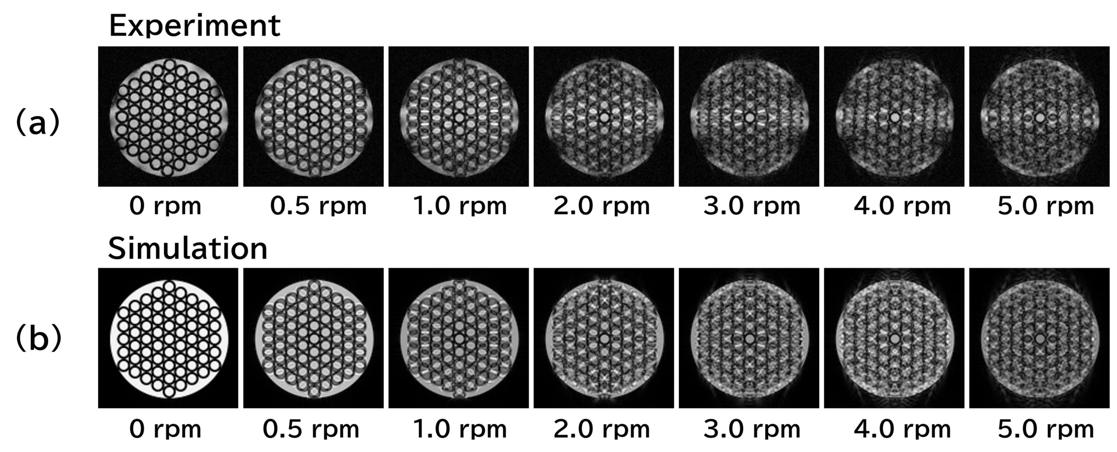
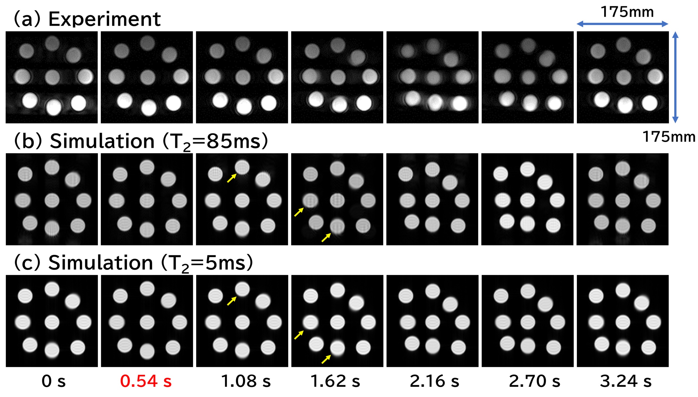
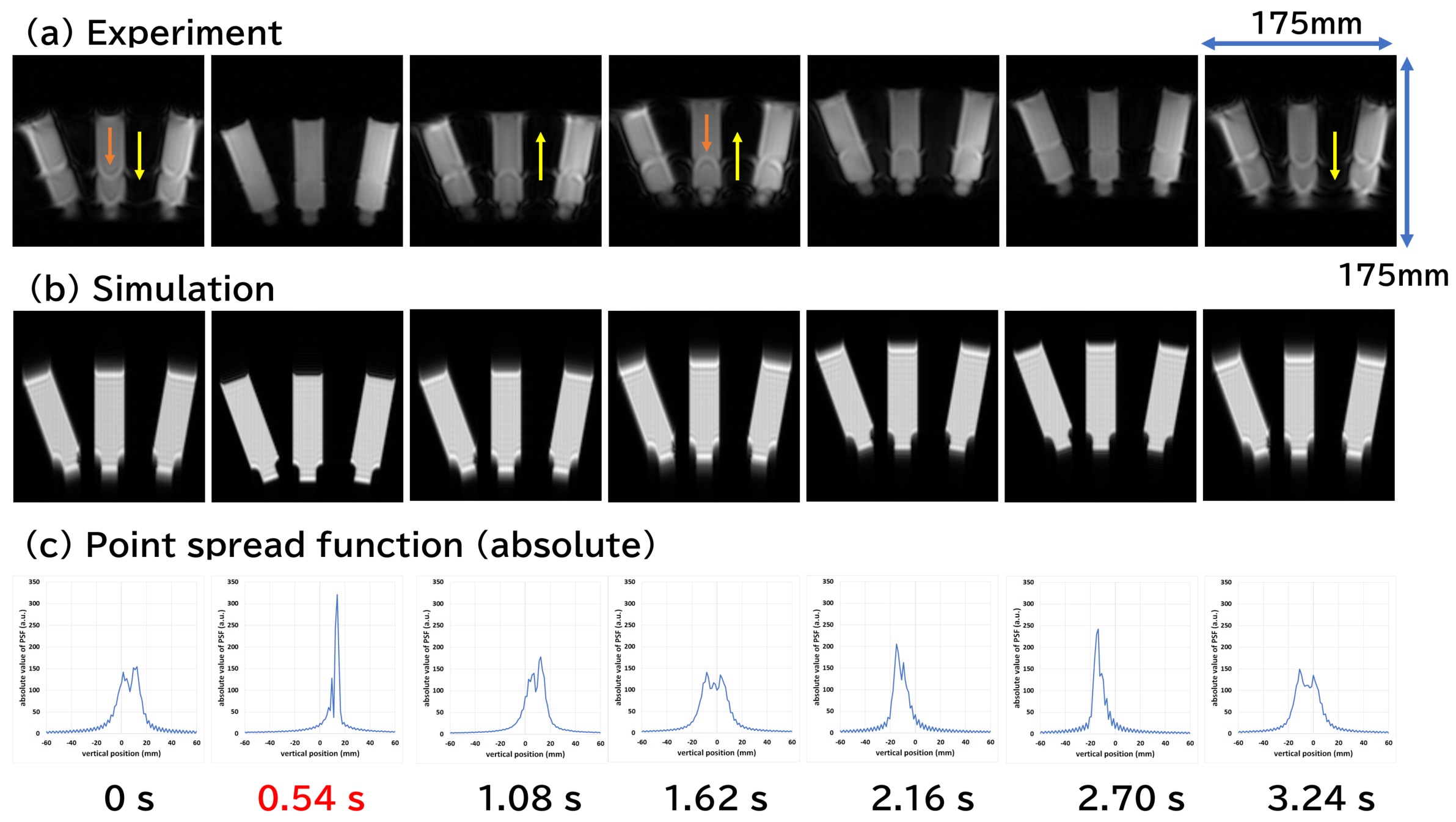
Figure 3 shows cross-sections of the rotating phantom acquired with the experiment and the Bloch simulation. The calculation time for one image was about 4 minutes. Except for the inhomogeneity of the RF magnetic field effect, motion artifacts are reproduced almost exactly. Figure 4 shows axial images of the moving phantom acquired with the experiment and the Bloch simulation. T₂ values of 85 ms and 5 ms were used for the Bloch simulation. The calculation time for 8 images were about 16 hours. The blurred image of the container in the experiment is not reproduced in the simulation, but the position of the containers is accurately reproduced. Artifacts were seen in the images calculated with T₂ of 85 ms, whereas they were almost nonexistent in the images calculated with T₂ of 5 ms. Figure 5 shows coronal images of the moving phantom acquired with the experiment and the Bloch simulation, and the absolute values of the point spread function (PSF) calculated along the direction of the translational motion. The calculation time for 8 images were about 3 hours. The PSF clearly demonstrates the presence of the artifacts shown in the simulated images.

Discussion

Bloch simulation based on the Lagrange description allowed us to obtain simulated images that can be compared with the experimental images for moving objects. In the simulation of rotation, the artifacts were reproduced almost accurately. On the other hand, in the simulation of translation, it was possible to reproduce the position of the translational object, but it was difficult to reproduce the detailed artifacts. The reason why artifacts could not be reproduced may be due to insufficient experimental setting of the moving object and/or imperfection of the imaging system (eddy current effects, etc.). The artifacts associated with the inhomogeneity of the magnetic susceptibility distribution may be caused by a special magnetic field distribution in the sample. Therefore, more precise calculations will be required to reproduce them. In the Lagrange description, unlike the Euler description, the positions of the spins vary with time, which reduces the effect of T₂ coherence. Therefore, in the Bloch simulation, it is necessary to use a shorter T₂ value than the measured T₂. In conclusion, the Lagrange description can reproduce MR images of moving objects, but more careful calculations are needed to reproduce the detailed artifacts.

Acknowledgements

No acknowledgement found.