Synopsis

Keywords: Pulse Sequence Design, New Trajectories & Spatial Encoding Methods, Spiral, WHIRL, analytical

This work introduces exact time-dependent analytical solutions, for both gradient waveforms and k-space trajectories, for an optimized spiral-based imaging strategy based on maximum frequency, perpendicular slew rate, and gradient magnitude constraints.

Introduction

For those interested in implementing Spiral MRI, this work gives exact analytic expressions for both the gradient waveform and the k-space trajectory as a function of time for the WHIRL variant of spiral ^[1], dubbed WHIRL Encoding Described by Piecewise Exact Analytical Solutions (WHIRLED PEAS). Unlike previous analytical approximate solutions for Archimedean spiral gradients waveforms ^[2,3], this work also adds a frequency-limited regime along with a slew-limited and gradient limited regime, similar to a previous numerical solution. ^[4]

Theory

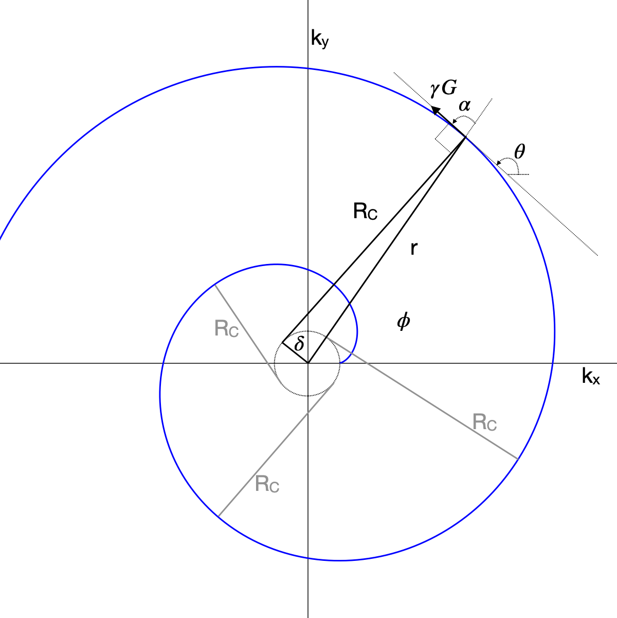
One can visualize the theory of WHIRLED PEAS in Fig. 1. Treating {k_x,k_y} as the complex plane, one can write

$$ \begin{align}
g&=Ge^{i \theta} \tag{1}\\
k&=re^{i \phi} \tag{2}\\
\alpha&= \theta - \phi \tag{3}\\
\delta&=\frac{N}{2 \pi F} \tag{4}\\
cos(\alpha) &= \frac{\delta}{r} \tag{5},
\end{align} $$

where g is the complex gradient waveform, k is the k-space location of the trajectory, $$$\alpha$$$ is the gradient angle from the radial direction, and $$$\delta$$$ is the radial distance in k-space at which N arms spanning 2$$$\pi$$$ will be the Nyquist distance 1/F apart from each other, where F is the FOV. The WHIRL spiral is defined outside of $$$\delta$$$ purely by enforcing Eq. (5) ^[1] Because of this difference from the conventional Archimedean spiral, which enforces $$$tan(\alpha)=(r/\delta)$$$ ^[4], one can easily solve for exact, time-dependent solutions by deriving

$$ \begin{align}
\theta ' &= \frac{\gamma G}{R_C} = \frac{S_{\perp}}{G} \tag{6}\\
R_C &= \sqrt{r^2-\delta^2} = \delta \theta \tag{7},
\end{align} $$

where R_C is the Radius of curvature for the gradient at any point (see Fig. 1), and $$$S_{\perp}$$$ is the part of the slew rate orthogonal to the gradient direction, i.e. $$$G \theta '$$$ (while the parallel component $$$S_{||}$$$ = G'). Note in Fig. 1 that the turning radius corresponding to R_C is always tangential to the central circle of radius $$$\delta$$$. Also, importantly, WHIRL (Eq. (5)) is not defined for r<$$$\delta$$$, in which the trajectories must exceed the Nyquist limit.

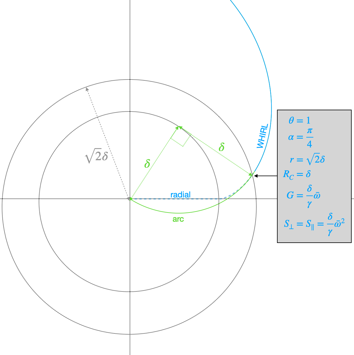
The initial path to WHIRLED PEAS, for this region, is shown in Fig. 2. This path is redefined, compared to reference (1), to be a quarter-circle arc with radius $$$\delta$$$. This arc is designed to meet the WHIRL trajectory at a radius of r=$$$\sqrt{2} \delta$$$, and $$$\theta$$$=1. Knowing the relevant variables for the WHIRL trajectory at this point (shown in gray box in Fig. 1) allows one to create an appropriate gradient waveform that matches the gradient, slew, and k-space waveforms smoothly between the arc and the WHIRL trajectory. Past this initial arc, the WHIRL trajectory is defined in three parts. These correspond to constraints from a maximum frequency $$$\bar{f}$$$ (or angular frequency $$$\bar{\omega} = 2 \pi \bar{f}$$$), a maximum orthogonal slew rate $$$\bar{S_{\perp}}$$$, and a maximum gradient amplitude $$$\bar{G}$$$, which ends when one reaches the maximum k-space radius $$$\bar{r}$$$. An entire set of trajectories is illustrated in Fig. 3.

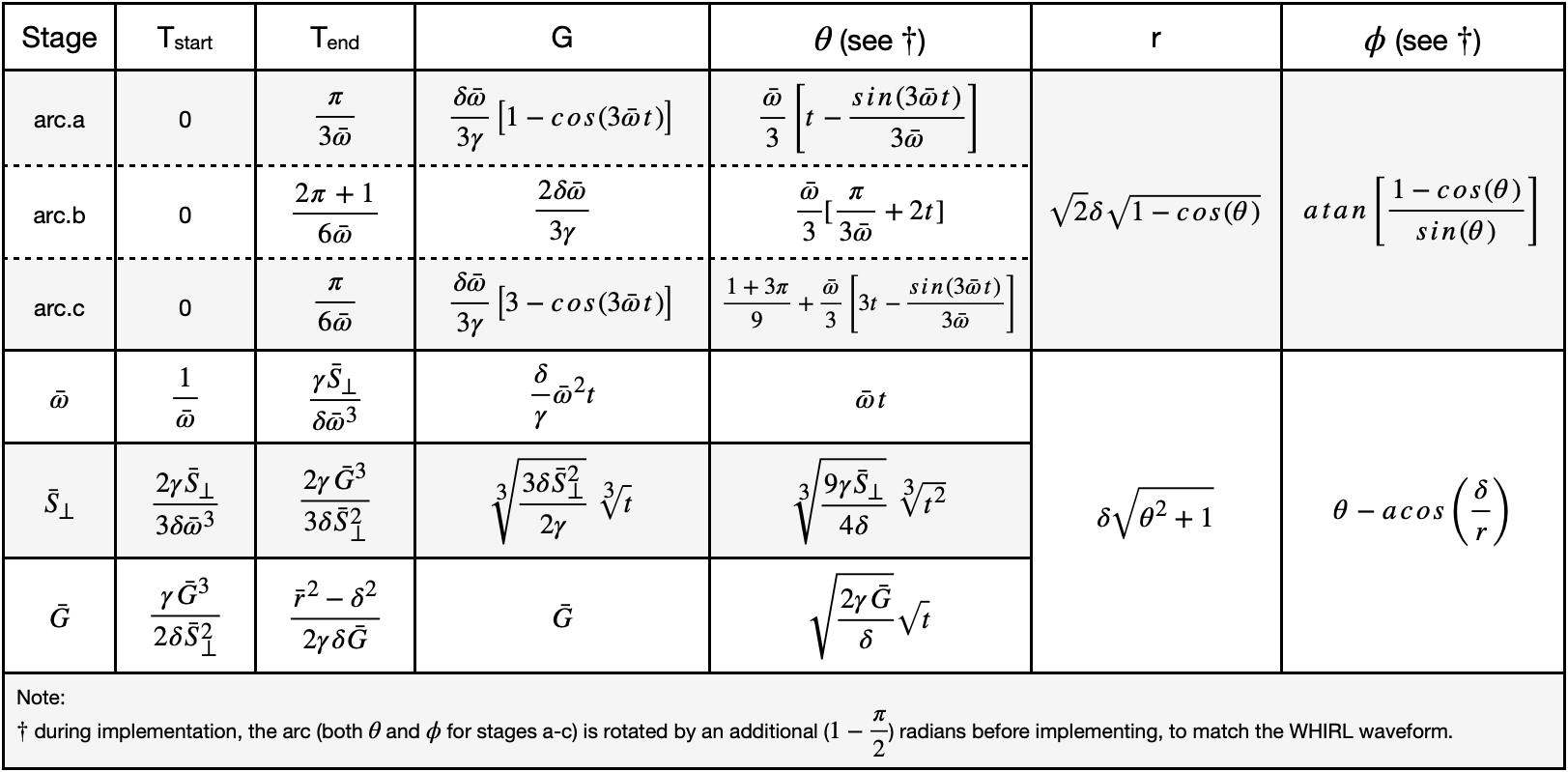
One can achieve WHIRLED PEAS under these constraints using the equations in Table 1. These are written as sections that are played back-to-back, with the time variable t in each section going from T_start to T_end. A plot of gradient waveforms, and one resulting spiral arm, are shown in Fig. 4. In each section there are analytical equations for both the gradient and k-space vectors, which allows each to be directly determined with its own dwell time. When, for any WHIRL section, T_end < T_start, this signifies that this section will be skipped - this is easily implemented by lowering the relevant constraint to make T_end = T_start.

Discussion

The analytical nature of the waveforms and durations (T_end-T_start) of each section allows one to appreciate the affects of different constraints on the gradient waveform and trajectory. The waveforms are similar to earlier forms [2,3], however are now exact matches for a constraints of the WHIRL spiral trajectory, include a section for constraint by a maximum frequency (useful to take gradient system frequency responses into account), and include convenient equations for k-space trajectories. The WHIRL trajectory keeps the normal distance between arms exactly constant, which the Archimedean spiral does not ^[1], and in that sense can be considered (slightly) more optimal, provided one finds a suitable initial path in innermost region of k-space, in which WHIRL is not defined.

It is noted that the slew constraint is $$$S_{\perp}=G \theta'$$$ only, not the total slew magnitude; however this typically represents 99% or more of the total slew on either side of this segment, and thus does not result in large jumps in slew between segments. Also, this work does not account for variable density spirals ^[5] or smoothed changes between segments ^[6].

Conclusion

This work introduces exact time-dependent solutions, for both gradient waveforms and k-space trajectories, for an optimized spiral-based imaging strategy based on maximum frequency, perpendicular slew rate, and gradient magnitude constraints.

Acknowledgements

This work was funded in part by Philips Healthcare.

References

[1] Pipe, J.G., An optimized center-out k-space trajectory for multishot MRI: Comparison with spiral and projection reconstruction. Magn. Reson. Med. 1999 42: 714-720.

[2] Glover, G.H., Simple analytic spiral K-space algorithm. Magn. Reson. Med. 1999. 42: 412-415.

[3] Salustri C, Yang Y, Glover GH, Simple but Reliable Solutions for Spiral MRI Gradient Design, J Magn Res 1999. 140(2): 347-350,

[4] Pipe JG, Zwart NR. Spiral trajectory design: a flexible numerical algorithm and base analytical equations. Magn Reson Med. 2014 Jan;71(1):278-85.

[5] Kim, D.-h., Adalsteinsson, E. and Spielman, D.M. (2003), Simple analytic variable density spiral design. Magn. Reson. Med., 50: 214-219.

[6] Pipe JG, Borup DD. Generating spiral gradient waveforms with a compact frequency spectrum. Magn Reson Med. 2022 Feb;87(2):791-799.