2361
3D High Resolution MR Fingerprinting for prostate cancer1Department of Radiology, University of Michigan, Ann Arbor, MI, United States, 2Department of Biomedical Engineering, University of Michigan, Ann Arbor, MI, United States
Synopsis
Keywords: MR Fingerprinting/Synthetic MR, MR Fingerprinting, prostate cancer
We developed a 3D MR Fingerprinting method with B0 correction for imaging the prostate gland. T1 and T2 maps with the spatial resolution of 1 x 1 x 3 mm3 were obtained from phantom and in-vivo experiments, demonstrating the potential of performing accurate and high-resolution tissue quantification of prostate cancer.Introduction
The goal of this study is to develop a 3D MR Fingerprinting (MRF) method for high-resolution mapping of T1 and T2 relaxation times in the prostate gland. MRF is a quantitative MR technique that allows for simultaneous quantification of multiple tissue properties in a single scan [1]. 2D MRF at a resolution of 1 x 1 x 5 mm3 has been applied in the prostate gland for separating cancer from non-cancerous tissue in both peripheral and transition zones and for differentiating between low grade lesions and intermediate/high grade lesions in the peripheral zone [2, 3, 4]. The maps obtained at this resolution require significant time expenditure and yet cannot be used for lesion detection, which limits the ability to incorporate such an acquisition into the clinical workflow. It is hoped that a high resolution, 3D MRF acquisition for the prostate can be used eventually for lesion characterization and detection. In this study, we developed a 3D MRF-FISP method using a stack-of-spirals (SoS) readout with B0 correction for imaging the prostate gland at a 1 x 1 x 3 mm3 resolution without zero-filling.Methods
A 3D MRF-FISP acquisition with the SoS readout was implemented. A total of 1000 image time points (TP) were acquired for each partition using a fixed TR of 12 ms, TE of 1.5 ms, and variable flip angles [5]. Each TP was highly undersampled with one of the 48 spiral arms that was designed for 1 mm2 in-plane spatial resolution for a field-of-view of 400 mm2. The total acquisition time for 32 partitions was 8 minutes. A dictionary of potential signal evolutions (30,105 entries) was calculated with ranges of T1 values between 10 and 5000 ms and T2 values between 2 and 800 ms using Bloch equation simulations.An inverse Fourier Transform along the partition direction was first performed on the 3D k-space data, then the 3D volume was compressed into 6 coefficient volumes using dictionary-based SVD compression [6]. After deblurring [7] using a field map from a GRE scan with two TEs (2.12 ms and 4.58 ms), the spiral data were gridded into images using NUFFT [8]. Finally, T1 and T2 maps were retrieved by taking the maximum of the cross-correlation between the reconstructed images and the dictionary. All experiments were performed in a Siemens Magnetom Vida 3T (Siemens Healthineers, Erlangen, Germany) with an 18-channel body array and a spinal array with 32 channels.
The NIST phantom [10] was scanned to assess the performance of the proposed method and the effect of B0 correction on T1 and T2 quantification.
Two volunteers were scanned using the proposed method and T2-weighted images were also acquired on each volunteer.
The study was approved by the institutional review board and informed written consent was obtained from all participants.
Results
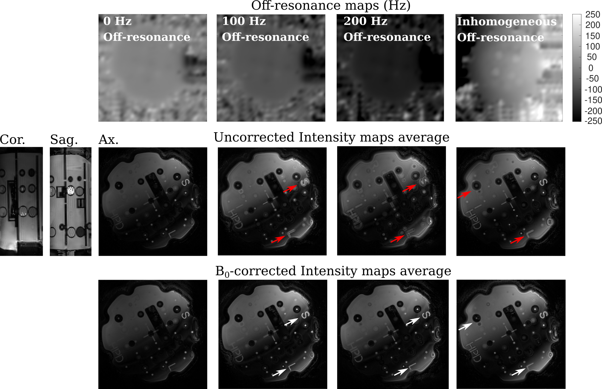
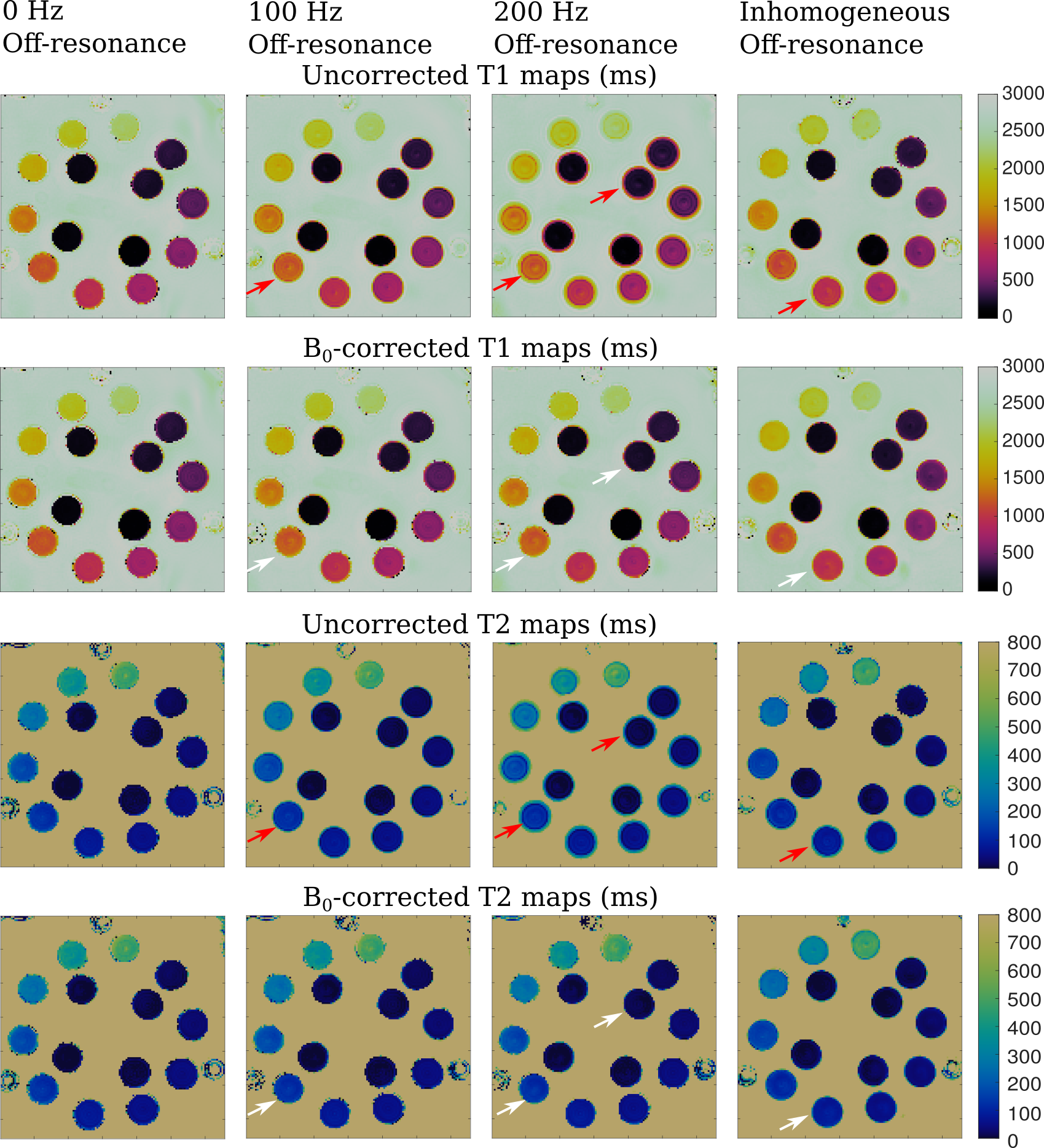
Fig. 1 shows a qualitative assessment of the deblurring algorithm on images acquired using the proposed sequence in the NIST phantom. Field maps with different off-resonance are shown in the first row, and the first coefficient images of one partition before and after the B0 correction are shown in 2nd and 3rd rows.In Fig. 2, the T1 and T2 maps of the T2 layer of the NIST phantom with and without B0 correction are displayed. A qualitative improvement after applying B0 correction is appreciated in the spheres where the applied off-resonance was higher.
Red arrows in Figs. 1 and 2 point out regions where the off-resonance blurring is significant. Same regions are pointed out in white arrows after applying B0 correction.
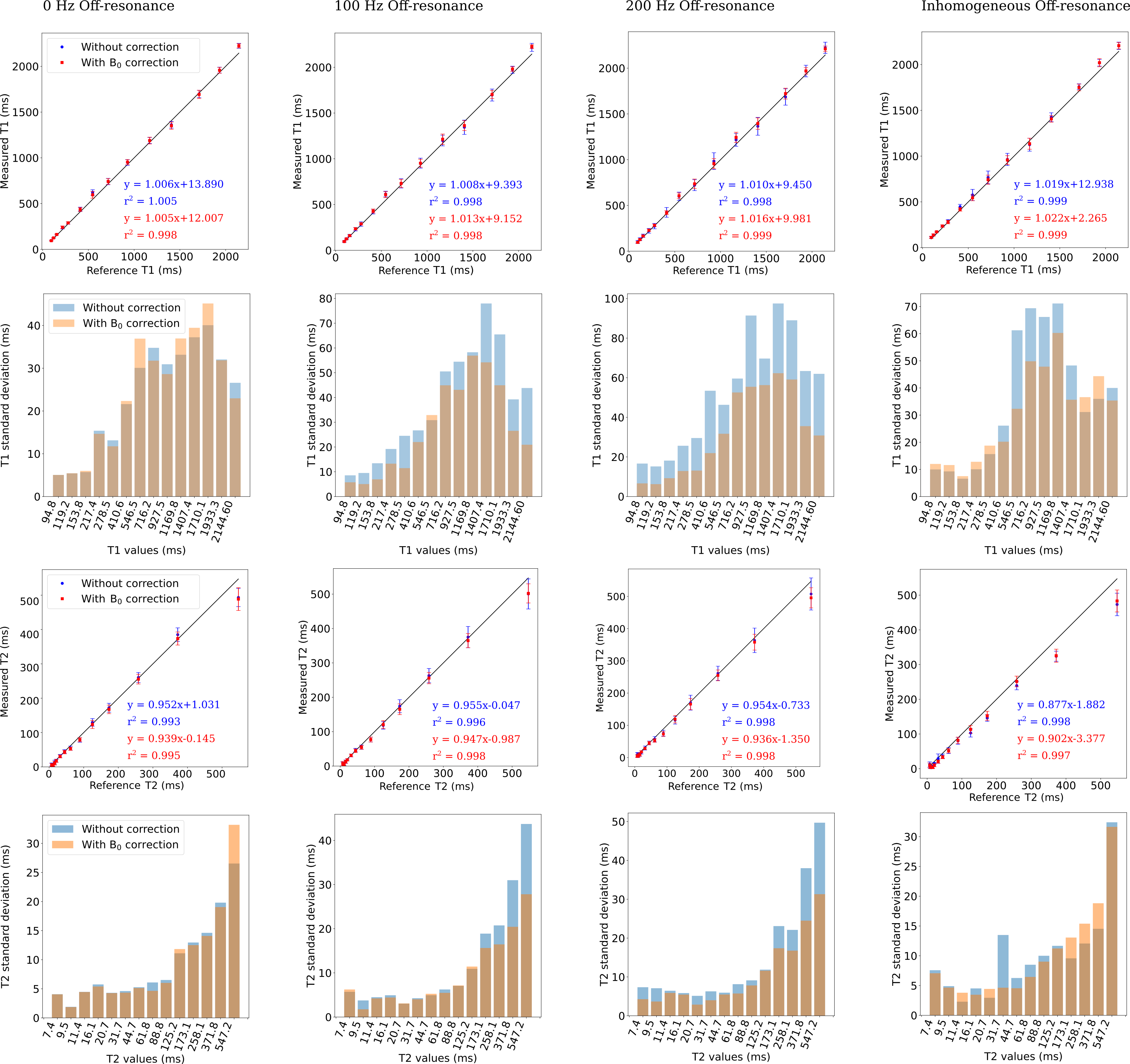
Fig. 3 shows correlation plots and their corresponding standard deviations of T1 and T2 values generated by the 3D-MRF-FISP sequence against the reference T1 and T2 values in the spheres shown in Fig. 2. A notorious reduction on the standard deviation was observed in both T1 and T2 values after applying B0 correction, particularly in spheres with relatively high off-resonance values.
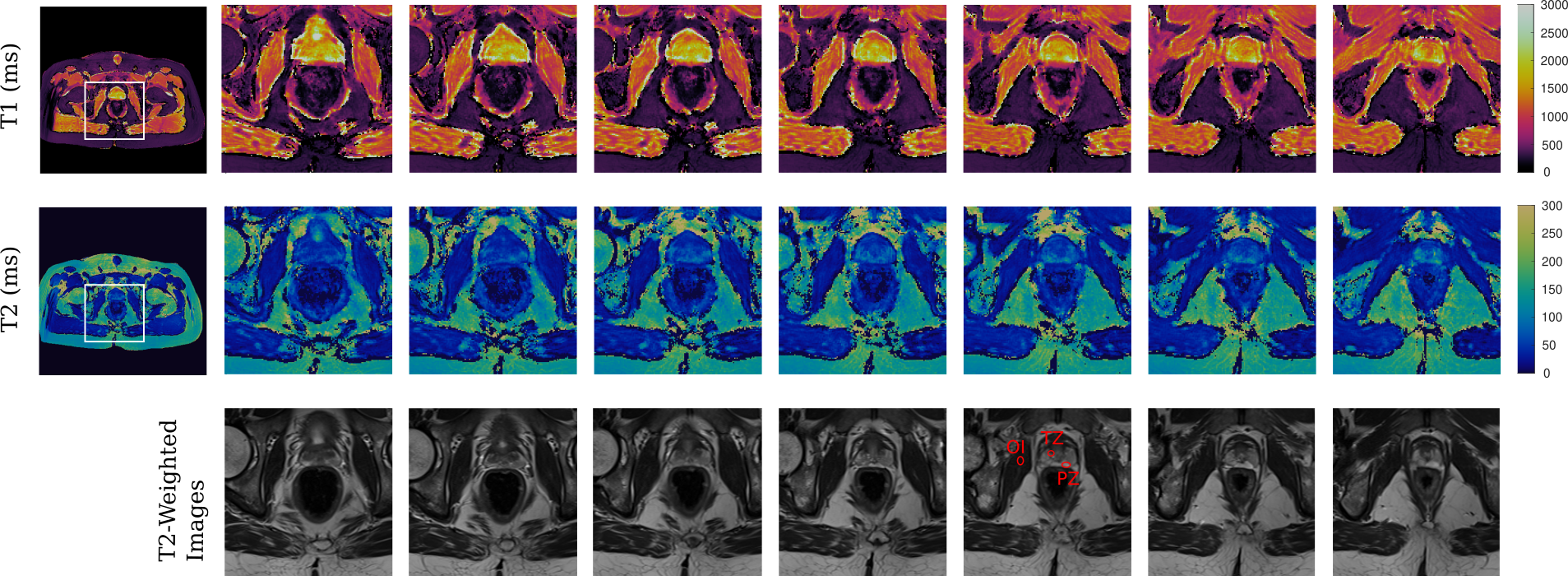
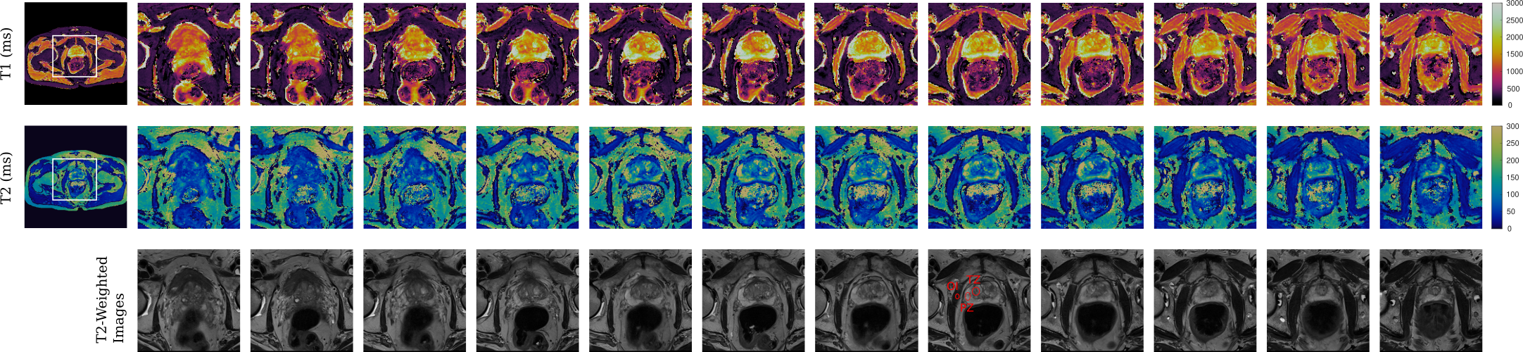
T1 and T2 maps of the prostate gland and their corresponding T2-weighted images from a 35 yr. volunteer are shown in Fig. 4. T1 And T2 maps of the whole pelvis are shown in the left side for a selected partition, pointing out with a white square the region-of-interest (ROI) over which the zoom was applied to. Same is displayed for a 75 yr. volunteer in Fig. 5. Quantitative T1 And T2 values (mean ± SD) are reported in Figures 4 and 5 for ROIs (red ellipses) drawn over the prostate peripheral zone (PZ), transitional zone (TZ), and the obturator internus (OI) muscle for both volunteers in a selected partition. These values are displayed in the figures captions. The values are between the expected ranges, respect to previously reported ones [2, 3, 4].
Conclusion and Discussion
In summary, we demonstrated the ability of a 3D MRF-FISP sequence to generate high-resolution (1 x 1 x 3 mm3) T1 and T2 maps of the whole prostate gland. It has the potential to improve the quantitative diagnostic capabilities using MRF and could be used for lesion detection. Further improvements such as B1 correction and regularization techniques over the intensity signals can be explored to find a more optimal combination of acquisition and reconstruction algorithms.Acknowledgements
Support for this study was provided by NIH grants R37CA263583 and R01CA208236, and Siemens Healthcare.References
1. Ma, D., Gulani, V., Seiberlich, N., Liu, K., Sunshine, J. L., Duerk, J. L., & Griswold, M. A. Magnetic resonance fingerprinting. Nature. 2013, 495(7440), 187-192.
2. Panda, A., Obmann, V. C., Lo, W. C., Margevicius, S., Jiang, Y., Schluchter, M., ... & Gulani, V. MR fingerprinting and ADC mapping for characterization of lesions in the transition zone of the prostate gland. Radiology. 2019; 292(3), 685.
3. Panda, A., O’Connor, G., Lo, W. C., Jiang, Y., Margevicius, S., Schluchter, M., ... & Gulani, V. Targeted biopsy validation of peripheral zone prostate cancer characterization with MR fingerprinting and diffusion mapping. Investigative radiology. 2019; 54(8), 485.
4. Yu, A. C., Badve, C., Ponsky, L. E., Pahwa, S., Dastmalchian, S., Rogers, M., ... & Gulani, V. Development of a combined MR fingerprinting and diffusion examination for prostate cancer. Radiology. 2017; 283(3), 729-738.
5. Jiang, Y., Ma, D., Seiberlich, N., Gulani, V., & Griswold, M. A. MR fingerprinting using fast imaging with steady state precession (FISP) with spiral readout. Magnetic resonance in medicine. 2015; 74(6), 1621-1631.
6. McGivney, D. F., Pierre, E., Ma, D., Jiang, Y., Saybasili, H., Gulani, V., & Griswold, M. A. SVD compression for magnetic resonance fingerprinting in the time domain. IEEE transactions on medical imaging. 2014; 33(12), 2311-2322.
7. Noll, D. C. Reconstruction techniques for magnetic resonance imaging. Stanford University. 1991; pp 108-114.
8. Fessler, J. A., & Sutton, B. P. Nonuniform fast Fourier transforms using min-max interpolation. IEEE transactions on signal processing. 2003; 51(2), 560-574.
9. Walsh, D. O., Gmitro, A. F., & Marcellin, M. W. Adaptive reconstruction of phased array MR imagery. Magnetic Resonance in Medicine: An Official Journal of the International Society for Magnetic Resonance in Medicine. 2000; 43(5), 682-690.
10. Keenan, K. , Stupic, K. , Boss, M. , Russek, S. , Chenevert, T. , Prasad, P. , Reddick, W., Zheng, J. , Hu, P. and Jackson. Comparison of T1 measurement using ISMRM/NIST system phantom, Proceedings of the International Society of Magnetic Resonance in Medicine, Singapore. 2016; https://tsapps.nist.gov/publication/get_pdf.cfm?pub_id=919826 (Accessed November 3, 2022).
Figures