2250
Development of Hepatocellular Carcinoma phantom and its use for assessing R2* mapping sequences for detecting iron sparing
Elisabeth Pickles1,2, Eleanor Cox3,4, Alison Telford2, Ferenc Mozes5, Gabriela Belsley5, Elizabeth Tunnicliffe5, Michael Brady2, Michael Pavlides5,6,7, Daniel Bulte1, and Susan Francis3,4
1Institute of Biomedical Engineering, University of Oxford, Oxford, United Kingdom, 2Perspectum Ltd, Oxford, United Kingdom, 3Sir Peter Mansfield Imaging Centre, University of Nottingham, Nottingham, United Kingdom, 4NIHR Nottingham Biomedical Research Centre, Nottingham University Hospitals NHS Trust and the University of Nottingham, Nottingham, United Kingdom, 5Oxford Centre for Magnetic Resonance, University of Oxford, Oxford, United Kingdom, 6NIHR Nottingham Biomedical Research Centre, University of Oxford, Oxford, United Kingdom, 7Translational Gastroenterology Unit, University of Oxford, Oxford, United Kingdom
1Institute of Biomedical Engineering, University of Oxford, Oxford, United Kingdom, 2Perspectum Ltd, Oxford, United Kingdom, 3Sir Peter Mansfield Imaging Centre, University of Nottingham, Nottingham, United Kingdom, 4NIHR Nottingham Biomedical Research Centre, Nottingham University Hospitals NHS Trust and the University of Nottingham, Nottingham, United Kingdom, 5Oxford Centre for Magnetic Resonance, University of Oxford, Oxford, United Kingdom, 6NIHR Nottingham Biomedical Research Centre, University of Oxford, Oxford, United Kingdom, 7Translational Gastroenterology Unit, University of Oxford, Oxford, United Kingdom
Synopsis
Keywords: Liver, Cancer
Survival rates for hepatocellular carcinoma (HCC) are poor, and improved methods for early detection are required. One such method may be the detection of iron sparing in HCC compared to the liver tissue using R2* mapping. We optimised sequences for the assessment of whole liver 3D R2* mapping, and developed a HCC phantom comprising small spheres with a range of R2* values to assess them. Agreement of the phantom R2* with reference values and between vendors, as well as the ability to detect small differences in R2* indicated the sequences have strong potential to detect iron sparing.Introduction
Survival rates from hepatocellular carcinoma (HCC), the most common primary liver cancer, are poor1 despite curative treatments being available2. Surveillance in at-risk individuals using ultrasound is recommended2–4, but ultrasound has only 23%5-47%6 sensitivity for early HCC detection. There is a need for a better surveillance tool. Several studies have shown iron is lower in HCC compared to surrounding liver tissue7–9. Since R2* can be used to estimate iron, this may allow early detection of such iron sparing in HCCs. However, multi-echo gradient echo (ME-GRE) sequences for R2* mapping have mainly been optimised to detect iron overload. We optimised 3D ME-GRE R2* mapping sequences for detection of iron sparing across two vendors, and built a ‘HCC phantom’ to represent R2* of iron in tumours and liver parenchyma to assess the sequences met requirements for detecting iron sparing.Methods
Requirements for detecting HCC iron sparing were defined to detect iron of 0-3 mg/g dry weight (dw)10, with localised differences in iron of 0.2 mg/g dw and higher10 in regions of 1 cm or more2. 3D ME-GRE sequences Siemens and Philips scanners were optimised at 3 T. Parameters are provided in Table 1.HCC Phantom The HCC phantom was developed, using solutions of MnCl2 and NiCl2 across 17 concentrations to modulate R2* and R111, with the Alam12 and Hankins13 equations used for conversion between R2* and iron concentration. 10, 15 and 20 mm diameter polypropylene spheres were filled with solutions with R2* to represent HCC iron concentrations. These spheres were attached to three plates within a hollow acrylic sphere (160 mm diameter) flood filled with a concentration to represent liver iron, see Figure 1A-C. The HCC phantom was scanned on both Philips and Siemens scanners using optimised 3D ME-GRE sequences.
Reference R2* values were obtained by scanning tubes (25 mm diameter, 115 mm height) filled with each concentration, placed in a water-filled tub (210 mm diameter, 160 mm height), using a 2D ME-GRE sequence on the Philips scanner (see Table 1), robust against artifacts due to its thin slice thickness and repetitions to increase signal-to-noise ratio. R1 was measured using a 5(3)3 MOLLI scheme.
Analysis T2* and R2* maps were generated using the MAGO method14. A 10/7.5/5 mm diameter circular ROI was placed on each 20/15/10 mm sphere and a 10 mm ROI on the background. A 15 mm diameter circular ROI was placed on each tube. Median R2* was calculated for each ROI. Bland-Altman methods were used to compare R2* and equivalent iron of the HCC phantom spheres with reference values from the tubes, and between vendors. To assess the ability to detect differences in iron of 0.2 mg/g dw, the R2* of the 20 mm spheres were compared with adjacent background R2*.
Results
The tubes provided reference R2* values with equivalent iron concentration 0.4 mg/g dw – 2.0 mg/g dw (Figure 1B), whilst the HCC phantom background had equivalent iron concentration of 0.9 mg/g dw. R1 of the tubes ranged from 11 to 20 s-1, whilst the background was 14 s-1. R2* maps of the HCC phantom from each scanner are given in Figure 1D-E. Some spheres were excluded due to filling errors or could not be quantified, particularly on the Siemens data which appeared smoother. Bland-Altman plots show good agreement of R2* between vendors for the 20 mm spheres, whilst for the smaller spheres there were discrepancies between vendors at higher R2* values (Figure 2).Bland-Altman plots comparing R2* of the spheres with the reference tubes are given in Figure 3A. For the 20/15/10 mm spheres, the R2* bias from the reference was 2/-9/-12 s-1 on the Philips scanner and 1/-16/-10 s-1 on the Siemens scanner. For all sphere sizes, the limits of agreement were larger for Siemens than Philips. Bland-Altman plots comparing equivalent iron of the spheres with the reference tubes are given in Figure 3B. The 20 mm spheres were similar to equivalent iron of ±0.2 mg/g or less from the reference, whilst the 15 and 10 mm spheres had some differences greater than ±0.2 mg/g dw from the reference.
ROIs placed on the 20 mm spheres to compare concentrations 3, 4 and 5 to adjacent background showed no overlap in the interquartile ranges (Figure 4) and thus potential to detect localised differences in-vivo.
Discussion
The HCC phantom showed that the 3D R2* mapping sequences could be used to measure iron within the required range, with differences in iron of 0.2 mg/g dw detectable. The size of the sphere impacted the results: smaller 10 mm spheres had R2* further from the reference values or were not visible on the R2* maps, particularly on Siemens scanners, where the data appear smoothed compared to Philips despite an attempt to match sequence parameters, indicating that the sequences may not be suitable for detecting tumours of 10 mm or less.Conclusion
The HCC phantom allowed assessment of the sequences to study HCC for detecting iron sparing. These optimised R2* sequences are now being used in trials in patients with HCCs to assess the utility of the sequence as a surveillance tool.Acknowledgements
EP was supported by an Industrial Fellowship from the Royal Commission for the Exhibition of 1851. This project was performed as part of the DeLIVER Consortium, funded by CRUK.References
1. Yang JD, Hainaut P, Gores GJ, Amadou A, Plymoth A, Roberts LR. A global view of hepatocellular carcinoma: trends, risk, prevention and management. Nat Rev Gastroenterol Hepatol. 2019;16(10):589-604.2. Galle PR, Forner A, Llovet JM, et al. EASL Clinical Practice Guidelines: Management of hepatocellular carcinoma. J Hepatol. 2018;69(1):182-236.
3. Marrero JA, Kulik LM, Sirlin CB, et al. Diagnosis, Staging, and Management of Hepatocellular Carcinoma: 2018 Practice Guidance by the American Association for the Study of Liver Diseases. Hepatology. 2018;68(2):723-750.
4. Kokudo N, Hasegawa K, Akahane M, et al. Evidence-based Clinical Practice Guidelines for Hepatocellular Carcinoma: The Japan Society of Hepatology 2013 update (3rd JSH-HCC Guidelines). Hepatol Res. 2015;45(2):123-127.
5. Park HJ,Seo N, Kim SY. Current Landscape and Future Perspectives of Abbreviated MRI for Hepatocellular Carcinoma Surveillance. Korean J Radiol. 2022 Jun;23(6):598-614.
6. Tzartzeva K, Obi J, Rich NE, et al. Surveillance Imaging and Alpha Fetoprotein for Early Detection of Hepatocellular Carcinoma in Patients With Cirrhosis: A Meta-analysis. Gastroenterology. 2018;154(6):1706.
7. Ebara M, Fukuda H, Hatano R, et al. Metal contents in the liver of patients with chronic liver disease caused by hepatitis C virus: Reference to hepatocellular carcinoma. Oncology. 2003;65(4):323-330.
8. Tashiro H, Kawamoto T, Okubo T, Koide O. Variation in the Distribution of Trace Elements in Hepatoma. Biol Trace Elem Res. 2003;49.
9. Honda H, Kaneko K, Kanazawa Y, et al. MR imaging of hepatocellular carcinomas: Effect of Cu and Fe contents on signal intensity. Abdom Imaging. 1997;22(1):60-66.
10. Ebara M, Fukuda H, Kojima Y, et al. Small hepatocellular carcinoma: Relationship of signal intensity to histopathologic findings and metal content of the tumor and surrounding hepatic parenchyma. Radiology. 1999;210(1):81-88.
11. Stupic KF, Ainslie M, Boss MA, et al. A standard system phantom for magnetic resonance imaging. Magn Reson Med. 2021;86(3):1194-1211.
12. Alam MH, Auger D, McGill LA, et al. Comparison of 3 T and 1.5 T for T2∗magnetic resonance of tissue iron. J Cardiovasc Magn Reson. 2016;18(1).
13. Hankins JS, McCarville MB, Loeffler RB, et al. R2* magnetic resonance imaging of the liver in patients with iron overload. Blood. 2009;113(20):4853-4855.
14. Triay Bagur A, Hutton C, Irving B, Gyngell ML, Robson MD, Brady M. Magnitude-intrinsic water–fat ambiguity can be resolved with multipeak fat modeling and a multipoint search method. Magn Reson Med. 2019;82(1):460-475.
Figures
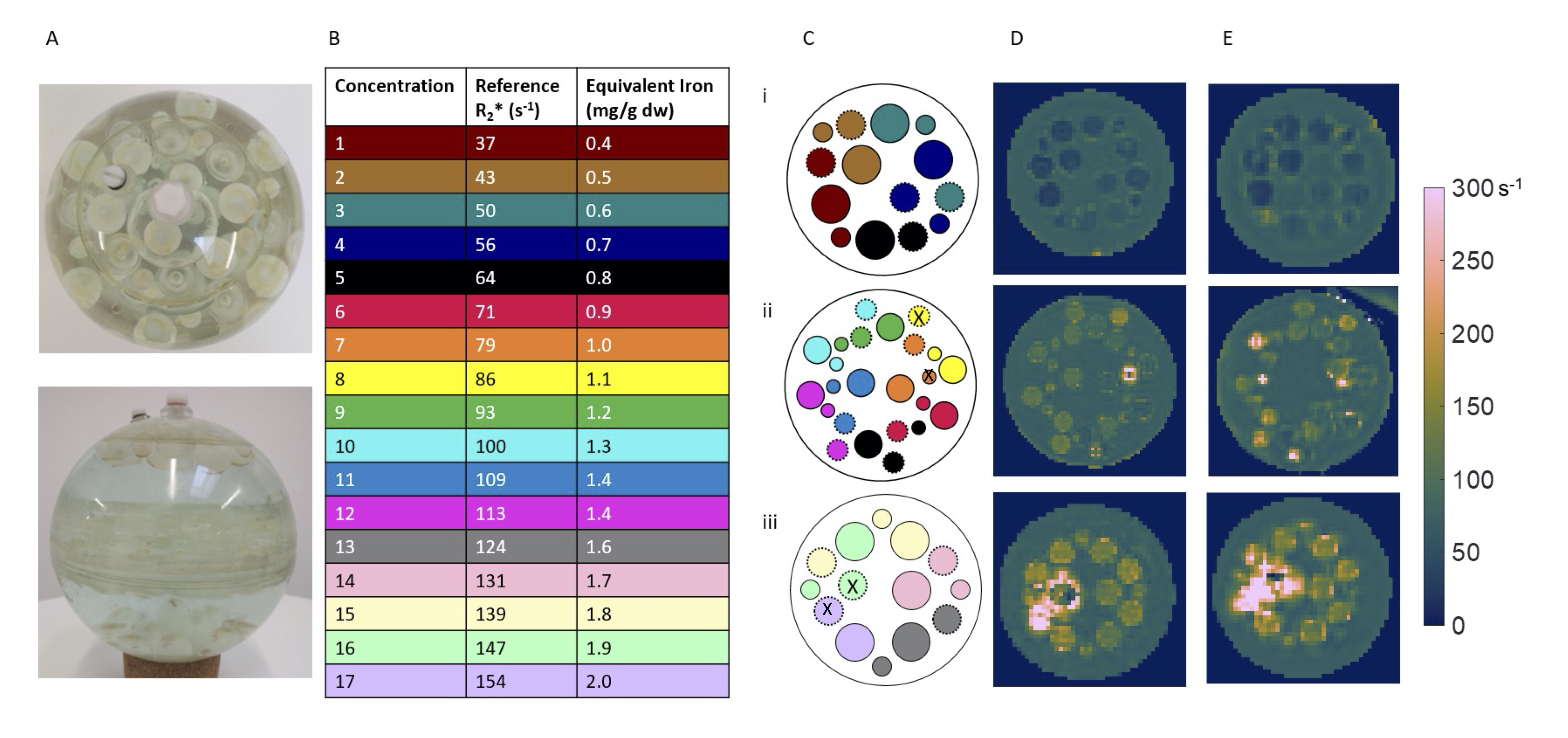
Figure 1: (A) Photographs of the HCC phantom. Colour-coded (B) reference tube concentrations and (C) schematic of the spheres in the phantom. [In the schematic: dashed outline = 15 mm spheres, spheres indicated by an X were excluded from analysis for both vendors due to filling errors or artifacts.] R2* maps for (D) Philips and (E) Siemens optimised sequence, for (i): Upper layer (ii) Middle layer (iii) Lower layer of spherical phantom.

Figure 2: Bland-Altman plots comparing R2* of the HCC phantom spheres between Philips and Siemens scanners. Those spheres which could not be quantified because they were missing, there was an artifact (areas of T2* shortening likely due to bubbles) or filling errors are excluded. Solid line = bias, dashed line = upper/lower 95% limit of agreement.
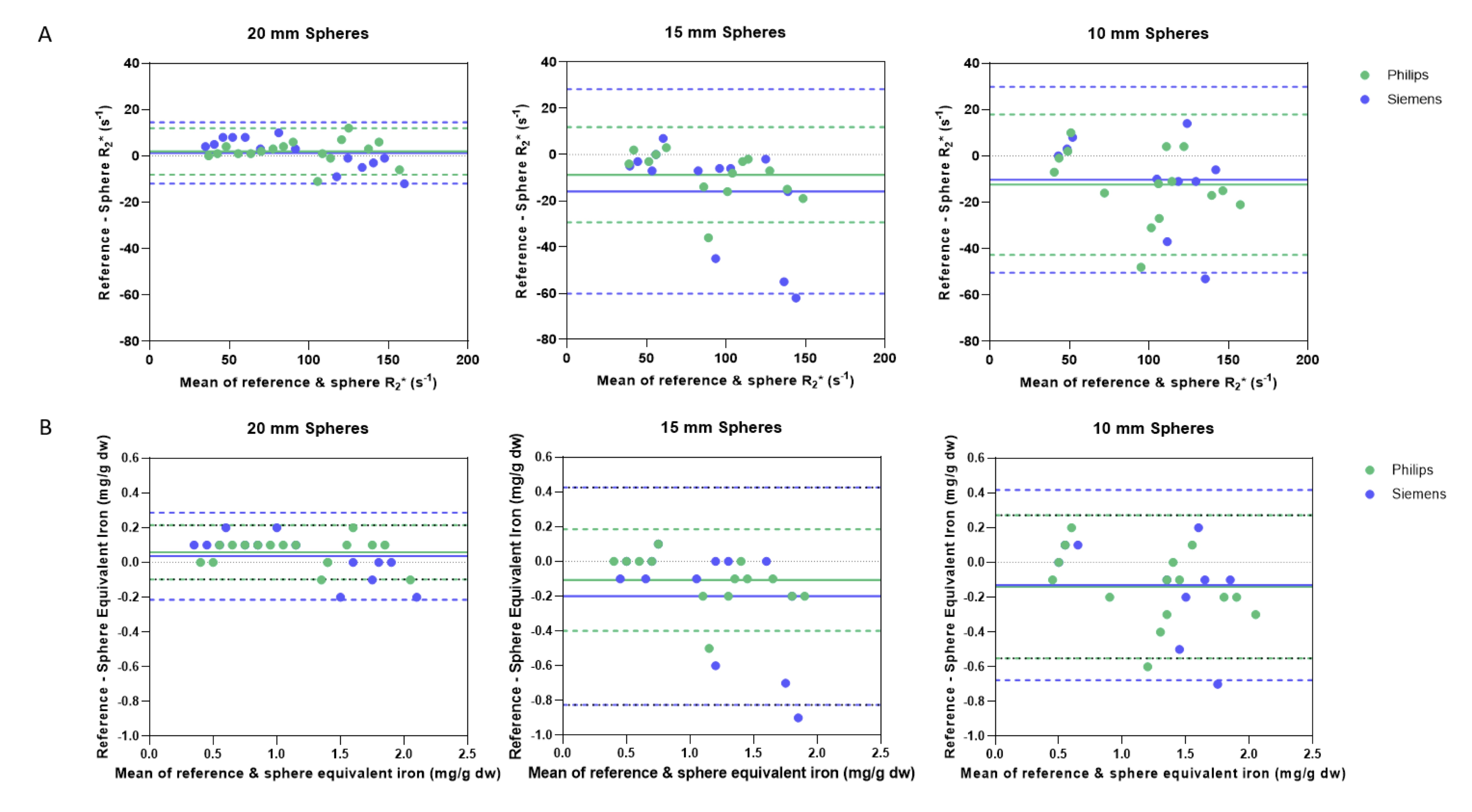
Figure 3: Bland-Altman plots comparing (A) R2* and (B) equivalent iron of the reference tubes with the HCC phantom spheres. R2* values were computed and converted into iron concentration using the Alam12 and Hankins’13 equations. Those spheres which could not be quantified because they were missing, there was an artifact (areas of T2* shortening likely due to bubbles) or filling errors are excluded. Solid line = bias, dashed line = upper/lower 95% limit of agreement.
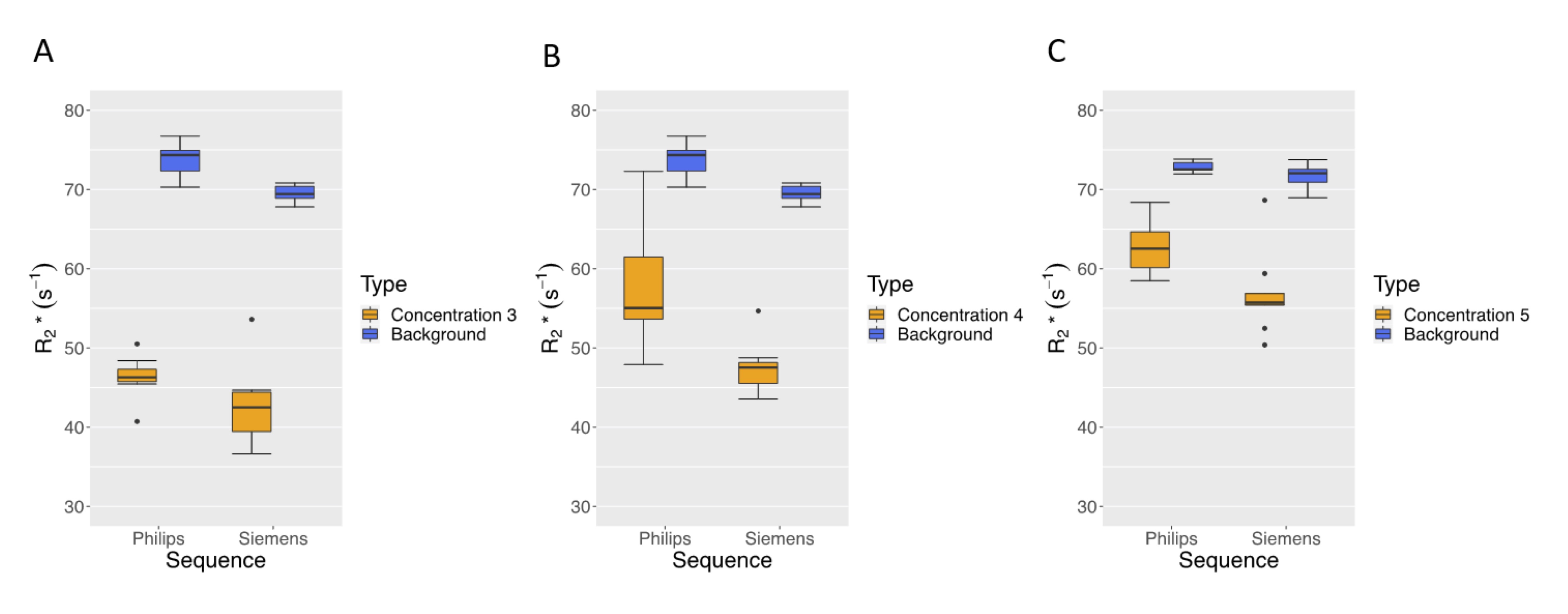
Figure 4: Comparison of 20 mm sphere R2* with background R2* for (A) Concentration 3 R2* equivalent to 0.6 mg/g dw iron, (B) Concentration 4 R2* equivalent to 0.7 mg/g dw iron and (C) Concentration 5 R2* equivalent to 0.8 mg/g dw iron. Background R2* equivalent to 0.9 mg/g dw iron. There was an area of higher R2* in the Philips Concentration 4 sphere, which was not present in the Siemens map, hence the larger range. This may have been due to a bubble in or near the sphere.
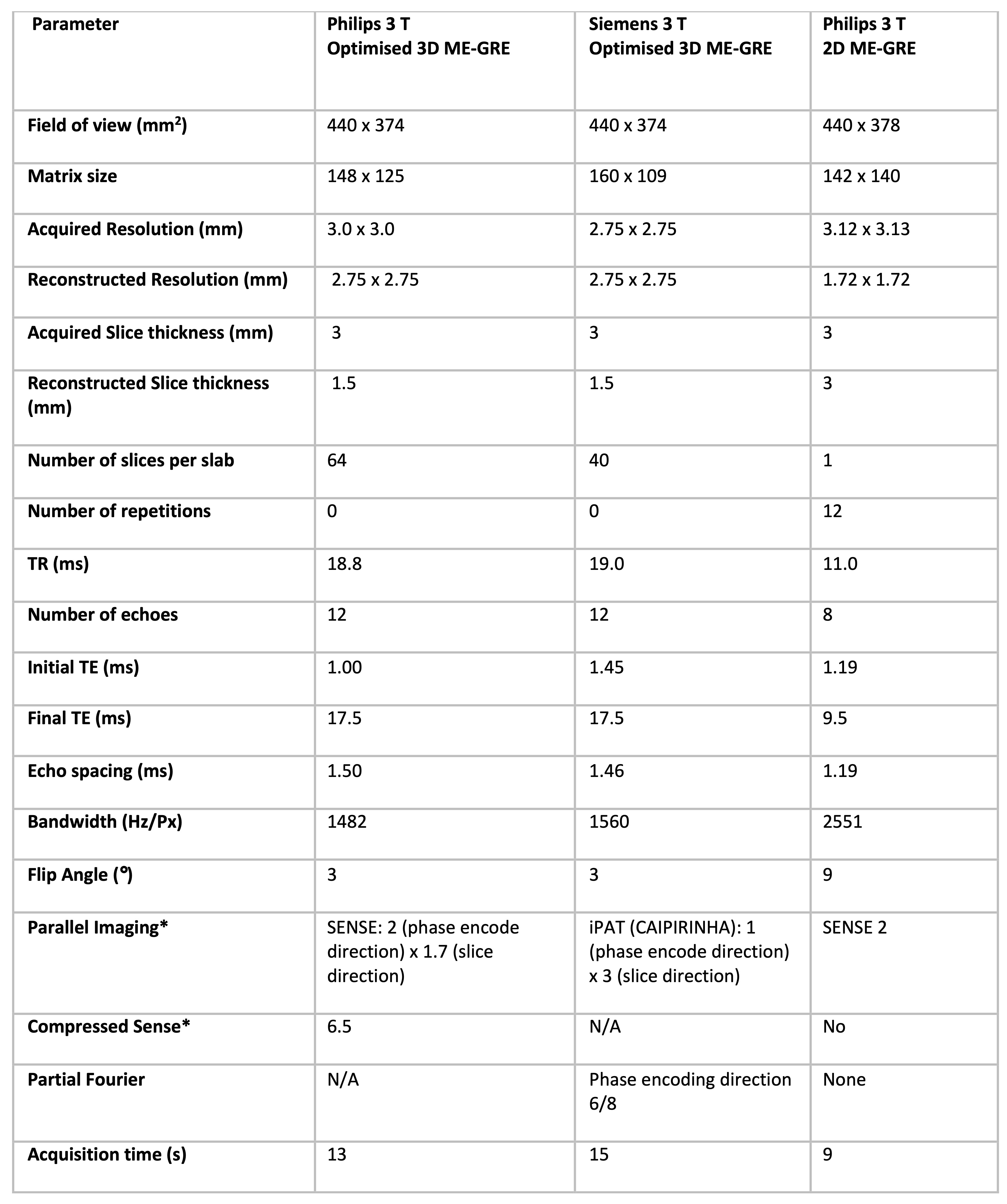
Table 1: Sequence parameters for optimised 3D ME-GRE sequence (Philips and Siemens) and the reference 2D ME-GRE sequence (Philips). *Note: Philips 3D ME-GRE protocols developed for SENSE and compressed SENSE, with data from the compressed sense protocol shown in this abstract.
DOI: https://doi.org/10.58530/2023/2250