2212
Analysis of the Discretization Error vs. Estimation Time Tradeoff of MRF Dictionary Matching and the Advantage of the Neural Net-based Approach
Chinmay Rao1, Jakob Meineke2, Nicola Pezzotti3, Marius Staring1, Matthias van Osch1, and Mariya Doneva2
1Leiden University Medical Center, Leiden, Netherlands, 2Philips Research, Hamburg, Germany, 3Philips Research, Eindhoven, Netherlands
1Leiden University Medical Center, Leiden, Netherlands, 2Philips Research, Hamburg, Germany, 3Philips Research, Eindhoven, Netherlands
Synopsis
Keywords: MR Fingerprinting/Synthetic MR, MR Fingerprinting
Traditional MR fingerprinting involves matching the acquired signal evolutions against a dictionary of expected tissue fingerprints to obtain the corresponding tissue parameters. Since this dictionary is essentially a discrete representation of a physical model and the matching process amounts to brute-force search in a discretized parameter space, there arises a tradeoff between discretization error and parameter estimation time. In this work, we investigate this tradeoff and show via numerical simulation how a neural net-based approach solves it. We additionally conduct a phantom study using 1.5T and 3T data to demonstrate the consistency of neural net-based estimation with dictionary matching.Introduction
Magnetic Resonance Fingerprinting (MRF) 1 is a quantitative MRI technique combining fast data acquisition with robust parameter mapping. One of its key enablers is dictionary-based parameter estimation. An MRF dictionary is a discrete representation of a physical model constructed by grid-sampling the parameter space. Naturally, there comes a tradeoff between grid density and matching speed. In neural network (NN)-based MRF parameter estimation 2-4, a trained NN model represents a continuous functional approximation of the inverse physical model and can, in theory, overcome the fundamental limitation of traditional matching. We show via numerical simulation that the NN-based approach is consistent with full dictionary matching (FDM) and that fast matching at the speed of the NN performed with a reduced dictionary (RDM) produces a predictable worst-case discretization error. Further, to strengthen the former result, we evaluate the agreement between NN and FDM on phantom data acquired using two field strengths.Methods
We used a sequence of 625 time points, TR=12 ms, TE=3 ms, and an optimized FA pattern 5. A dictionary of 308922 fingerprints was computed using Bloch simulation for a T1/T2 grid with T1 range 9-5056 ms, T2 range 5-2018 ms, and 2% grid spacing relative to T1/T2 values. The dictionary was compressed in time domain to 6 coefficients using SVD. A 6-layer complex-valued NN 3 was defined that accepts compressed fingerprints and outputs T1 and T2 parameters. To simulate realistic signal corruption for training, fingerprints were scaled by a random complex scaling factor with magnitude 0.4-2.4 and phase 0-2π. Complex Gaussian noise of σ=0.01 was added resulting in SNRmax range 40-240, where SNRmax is defined as the noise level relative to the MR signal from a fully relaxed spin system (with M0=1) excited by a 90° pulse 6. The fingerprints were normalized to have unit L2 norm. The dictionary was randomly split 90%-10% for training and validation. The NN model was trained using Cramér-Rao bound-weighted MSE loss 4 and Adam optimizer (0.001 learning rate, 512 batch-size, 500 epochs). For numerical simulation, first, the estimation time was defined as the time required to compute T1/T2 maps given a single-slice image series of size 224x224 and 6 coefficients. On Intel Xeon W-2235 CPU, FDM and NN inference required 23.4 s and 0.5 s, respectively. Then, a coarse dictionary was created with a 36x subsampled T1/T2 grid - 6x along each axis - which matched within the same time budget as our NN. We conducted in-dictionary and out-of-dictionary bias-variance analyses where 12 T1/T2 combinations were chosen from the reduced dictionary's grid and 12 from halfway between its grid points. In each case, 250 noisy realizations of fingerprints per T1/T2 combination were produced at 4 noise levels - SNRmax={50,100,150,200}. Estimation bias and variance of FDM, RDM, and our NN were calculated. For the phantom study, four scans of the T2-plane of an HPD System Phantom Model 130 7 were acquired using Philips Ingenia 1.5T/3T scanners with 15-channel head coil. All scans were in coronal orientation with 224 mm x 224 mm FOV, 1 mm x 1 mm in-plane resolution, and 4 mm slice thickness. A multi-slice spiral acquisition trajectory (5.9 ms window, 36 interleaves) was used to obtain k-space data for 15 slices. Coefficient images were reconstructed from the non-Cartesian k-space data using a non-iterative low-rank inversion method. For each series, T1/T2 maps were estimated for the central slice using FDM and our NN, and their probe-wise distributions were compared.Results and Discussion
In the in-dictionary simulation scenario (Figure 1), RDM was comparable to FDM at SNRmax=50. With increasing SNR, RDM's variance became slightly lower. This can be attributed to the greater noise contribution than the discretization's contribution (which is zero) to the variance. At SNRmax≥100, RDM's coarse T1/T2 grid offered greater isolation between signal noise and estimate variance resulting in more robust matching. In the out-of-dictionary case (Figure 2), while all three methods were comparable at SNRmax=50, RDM approached a fixed 6% standard deviation in higher T1 and mid-range T2 values at SNRmax≥100. This was expected considering the 6x reduction factor along the T1 and T2 grid axes of the reduced dictionary and because the out-of-dictionary T1/T2 values represented the worst-case off-grid points for RDM which maximized the contribution of discretization in the estimation variance. Thus, the drawback of RDM in the out-of-dictionary scenario outweighed its advantage in the in-dictionary case. In contrast, our NN was consistent with FDM in each case in terms of variance. In the phantom results (Figures 3, 4, and 5), a high agreement between our NN and FDM was observed for T1 and T2 at both 1.5T and 3T field strengths.Conclusion
T1/T2 estimation using an NN was not only comparable in precision to matching with a dense dictionary but also was 46x faster. To achieve fast matching, the dictionary had to be heavily subsampled by a factor of 36 thereby trading away its precision and demonstrating a fundamental limitation of dictionary matching. Estimation using a simulation-trained NN can replace FDM without significant change in estimation quality for scans of a standardized phantom at multiple field strengths. Future work will investigate the effect of discretization on in vivo data where the T1/T2 distribution is more heterogeneous.Acknowledgements
We would like to thank Kay Nehrke and Yoo Jin Lee for their support with data acquisition and pre-processing and Thomas Amthor for his support with the software implementation of the MRF physical model and dictionary matching.References
- Ma D et al., Nature. 2013 Mar; 495(7440):187-92.
- Cohen O et al., Magn Reson Med. 2018 Sep; 80(3):885-94.
- Virtue P et al., Proc IEEE ICIP. 2017 Sep; (pp. 3953-3957).
- Zhang X et al., Magn Reson Med. 2022 Jul; 88(1):436-48.
- Sommer K et al., Magn Reson Imaging. 2017 Sep; 41:7-14.
- Assländer J, J Magn Reson. 2021 Mar; 53(3):676-85.
- Stupic KF et al., Magn Reson Med. 2021 Sep; 86(3):1194-211.
Figures
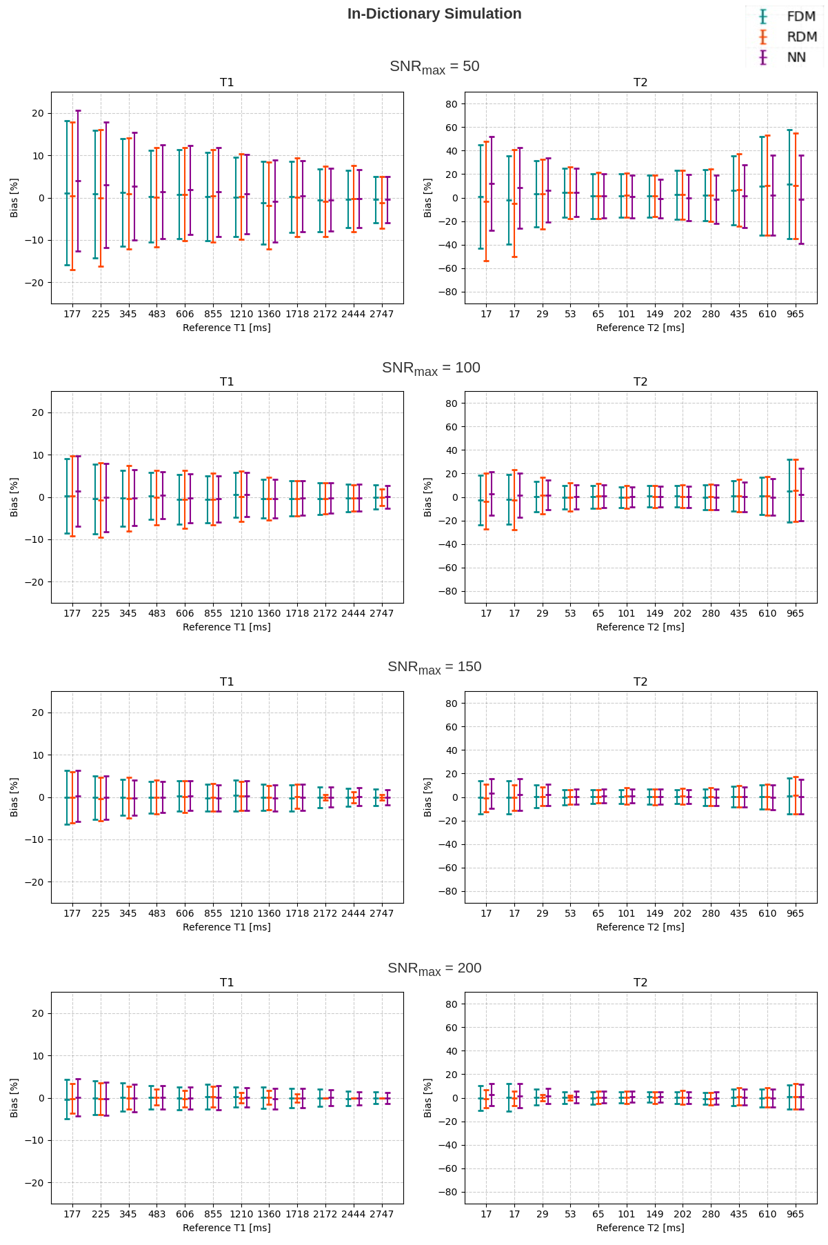
Figure 1: Bias-variance plots of T1 and T2 at different SNRmax levels for in-dictionary simulation. In each plot, bias is presented relative to the reference parameter value, and confidence intervals represent 1 standard deviation per side.
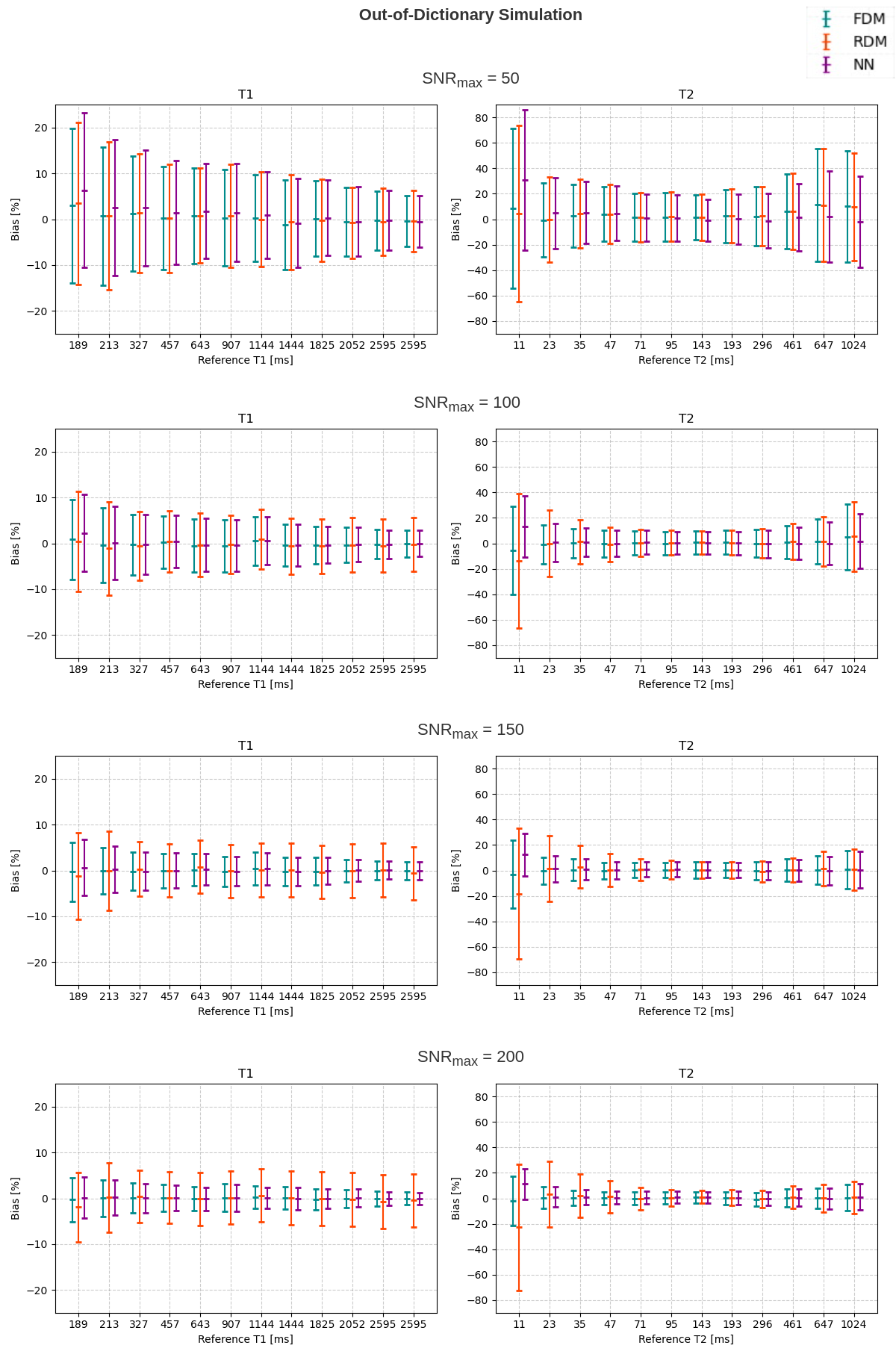
Figure 2: Bias-variance plots of T1 and T2 at different SNRmax levels for out-of-dictionary simulation. In each plot, bias is presented relative to the reference parameter value, and confidence intervals represent 1 standard deviation per side.
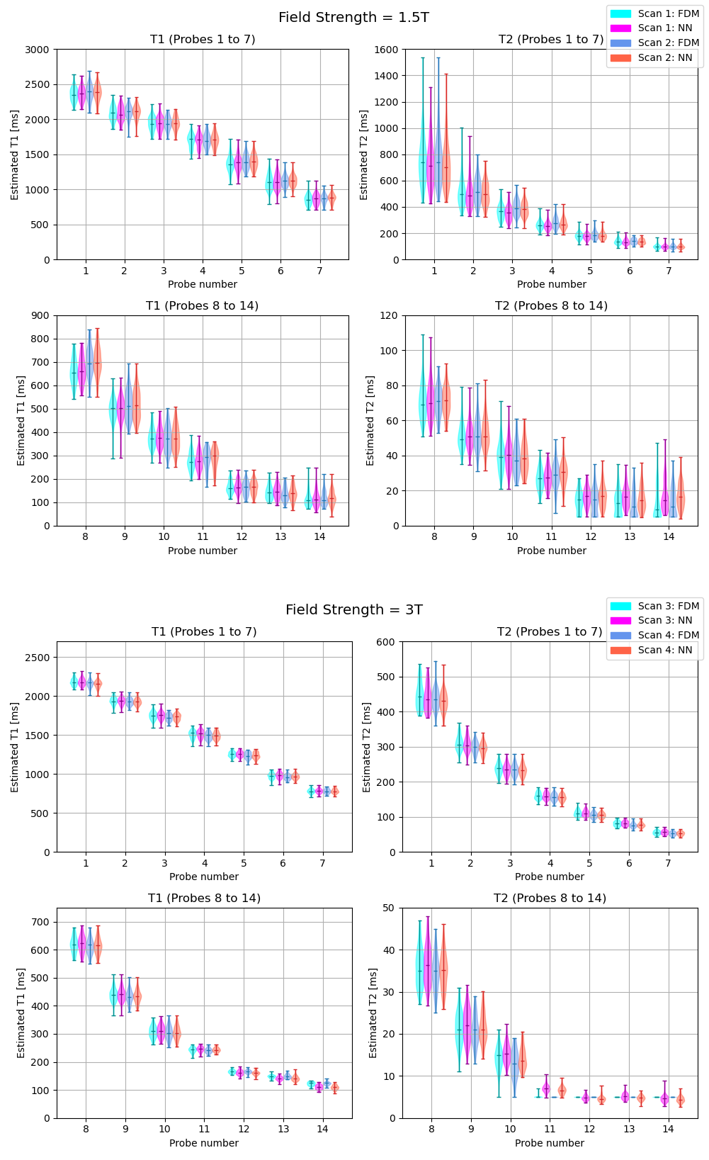
Figure 3: Probe-wise distribution of T1 and T2 estimates for 1.5T and 3T phantom data showing comparing NN with FDM. Scans 1 and 2 were acquired with 1.5T scanner whereas scans 3 and 4 with 3T scanner. For better visualization, results corresponding to the phantom's 14 probes are split into two parts - probes 1-7 and 8-14. Bars indicate estimation median and range.
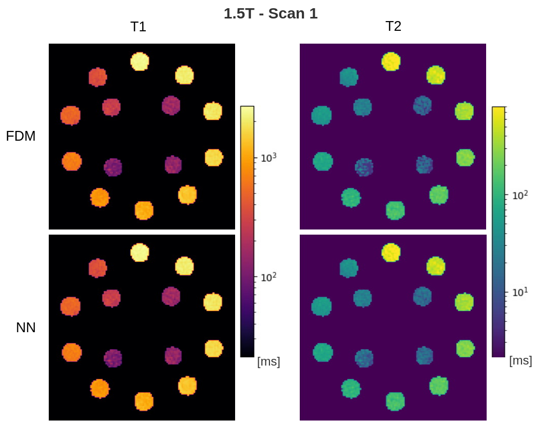
Figure 4: Estimated maps for 1.5T phantom scan 1. Background values are masked away to focus on the probes. Color scales are logarithmic.
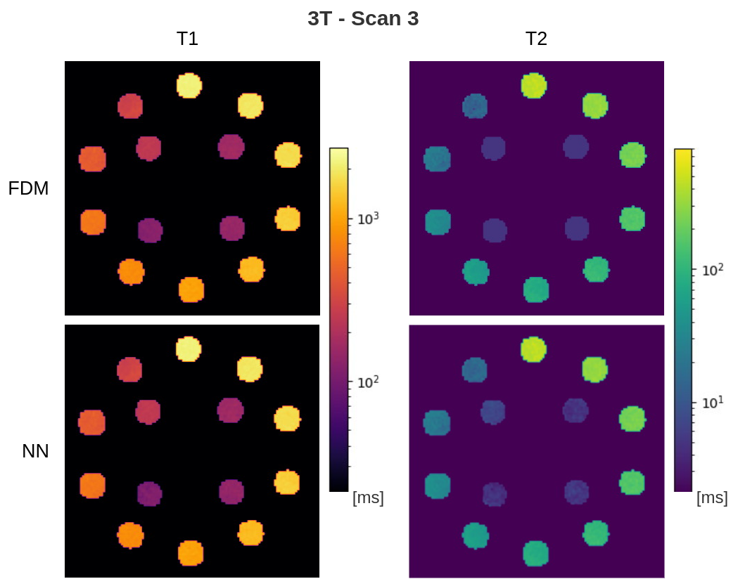
Figure 5: Estimated maps for 3T phantom scan 3. Background values are masked away to focus on the probes. Color scales are logarithmic.
DOI: https://doi.org/10.58530/2023/2212