2197
Cartesian MR-STAT vs spiral MR Fingerprinting: a comparison1Computational Imaging Group for MR Diagnostics and Therapy, Center for Image Sciences, University Medical Center Utrecht, Utrecht, Netherlands, 2Department of Radiology, Division of Imaging and Oncology, University Medical Center Utrecht, Utrecht, Netherlands, 3Philips Research, Hamburg, Germany
Synopsis
Keywords: MR Fingerprinting/Synthetic MR, Quantitative Imaging
MR Fingerprinting (“MRF”) and MR Spin Tomography in Time-domain (“MR-STAT”) are quantitative MRI techniques that allow multiple quantitative tissue parameter maps (e.g. T1, T2 and proton density) to be estimated from a single short scan. In this work, we compare the accuracy and precision of Cartesian MR-STAT and spiral MRF on gel phantoms and in-vivo. On gel phantoms we get excellent agreement with reference measurements. In-vivo we observe differences in reconstructed T1 values. As for the precision, a more in-depth study is required to take into account differences in noise-suppression mechanisms (i.e. k-space apodization and spiral sampling window).
Introduction
MR Fingerprinting1 (“MRF”) and MR Spin Tomography in Time-domain2 (“MR-STAT”) are quantitative MRI techniques that allow multiple quantitative tissue parameter maps (e.g. T1, T2) to be estimated from a single short scan. In MRF, spiral gradient trajectories are typically used, and parameters are estimated by matching “fingerprints” in each voxel separately to a pre-computed dictionary. In MR-STAT, Cartesian trajectories are typically used and parameters are estimated by iteratively solving a non-linear inversion problem for all voxels simultaneously. In this work, we compare for the first time the performance of 2D-spiral MRF and 2D-Cartesian MR-STAT on gel phantoms in terms of accuracy and precision of T1 and T2 estimates. We also evaluate the performance of both methods in-vivo and report on the challenges encountered when comparing the methods.Methods
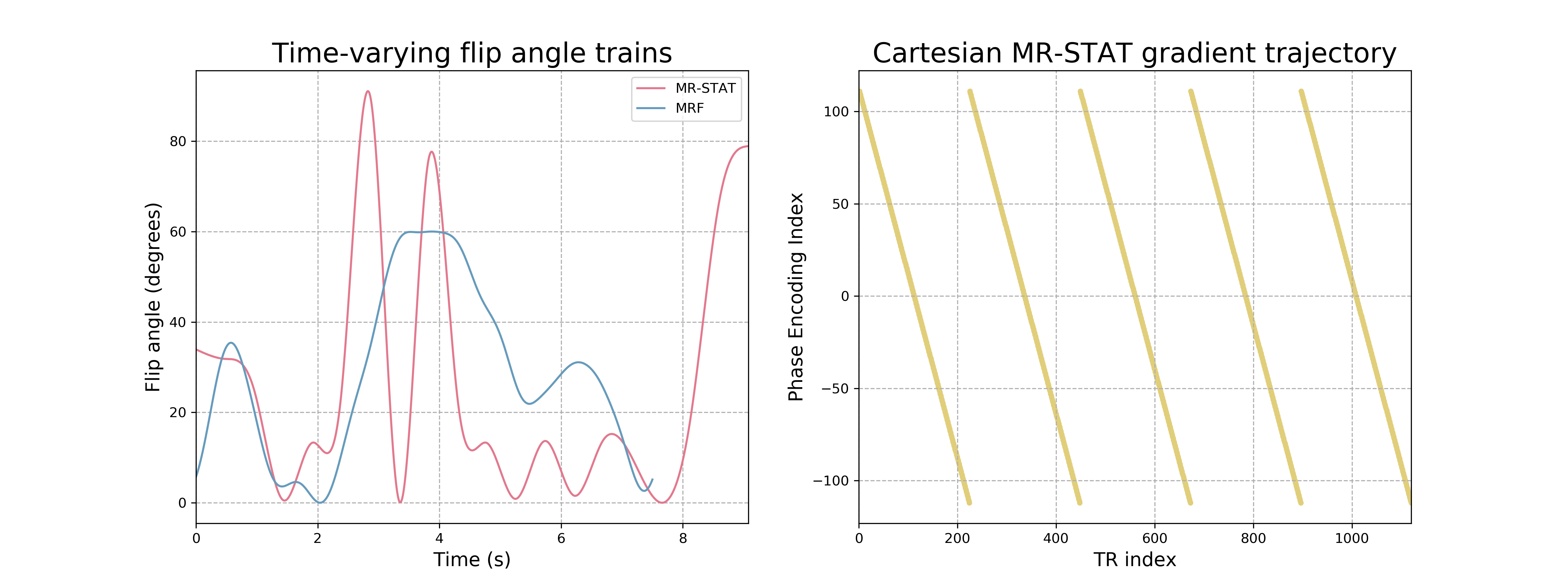
For both MRF and MR-STAT, gradient-spoiled gradient-echo pulse sequences with time-varying flip angles (Fig. 1a) were used to acquire data on 3T Ingenia Elition X clinical MR System (Philips Healthcare NV, Best, the Netherlands). In both the gel phantoms (TO5, Eurospin II test system, Scotland) and in-vivo scans (brain of a healthy volunteer) the field-of-view was set to 224 mm x 244 mm, with an in-plane resolution of 1 mm x 1 mm and a 4 mm slice thickness. The vendor’s 15-channel receive headcoil was used for signal reception.For MR-STAT, a 2D Cartesian gradient scheme was utilized where five fully-sampled “k-spaces” consisting of 224 readout lines each were acquired (Fig. 1b) with TR/TE = 8.18/3.97 ms, resulting in a scan time of 9.2 s. The readout bandwidth was 42.8 kHz with 224 samples per readout. The flip-angle train was generated using the BLAKjac technique3 (Fig. 1a) and was preceded by a non-selective adiabatic inversion pulse. The average power (i.e. the sum of the squared flip angles [degrees], divided by scan time [ms]) amounts to 155.1 [deg2/ms]. Reconstructions were performed using ten iterations of a matrix-free Gauss-Newton method.4
For MRF, 625 variable density spirals were acquired with TR/TR = 12.00/3.00 ms, resulting in a scan time of 7.5 s. The readout bandwidth was 287.4 kHz with 1668 samples per readout. The varying flip-angle train (Fig. 1a) and was preceded by a slice-selective adiabatic inversion pulse. The average power of the MRF sequence is 95.4 [deg2/ms]. For the MRF reconstruction, low-rank dictionary matching5 with rank 10 was used.
Both the gel phantom and in-vivo scans were repeated ten times to allow voxel-wise computation of standard deviations of the reconstructed T1 and T2 maps.
Single-echo (inversion recovery) spin-echo measurements were performed to obtain reference T1 and T2 values for the gel phantoms.
Results
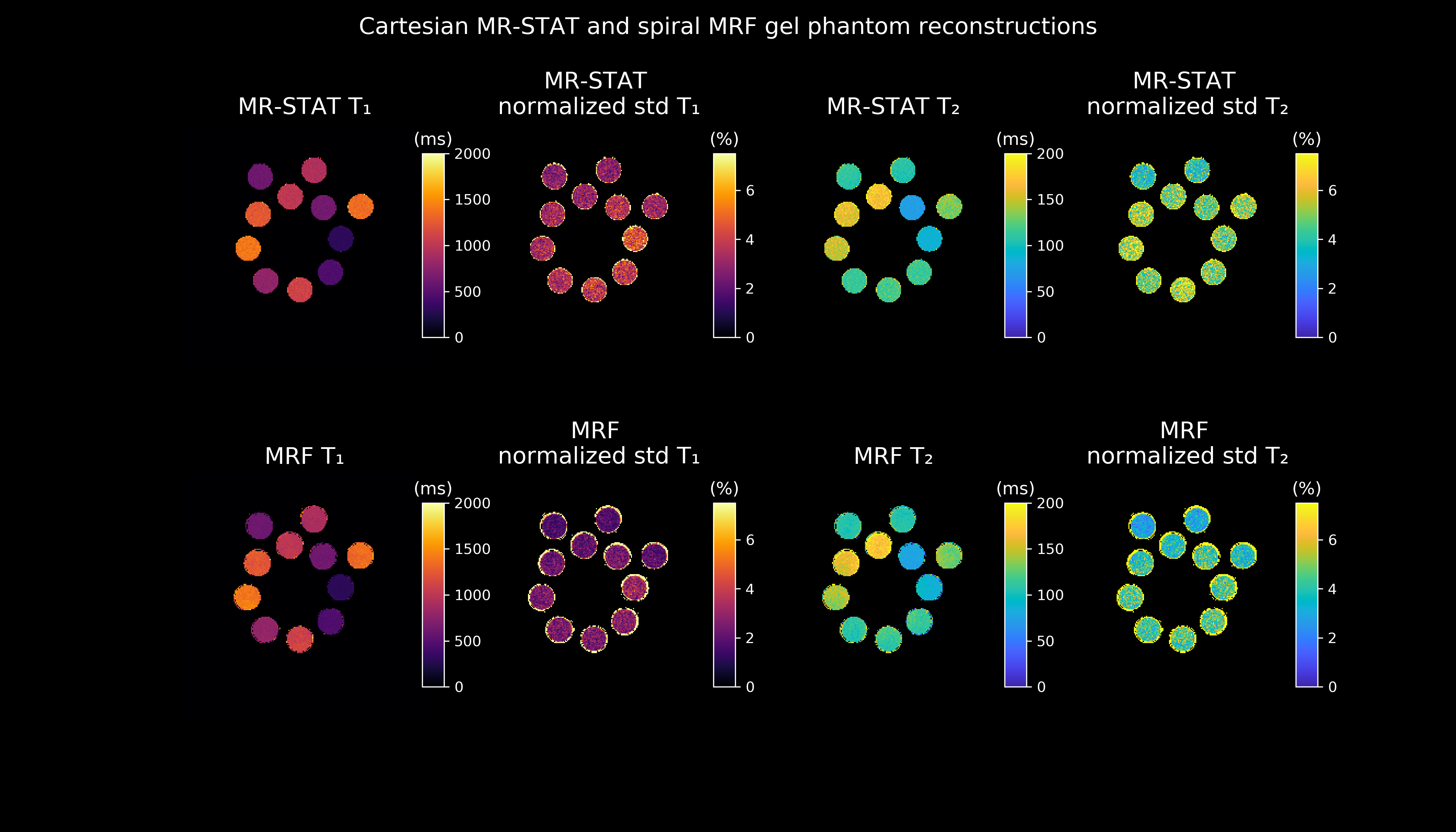
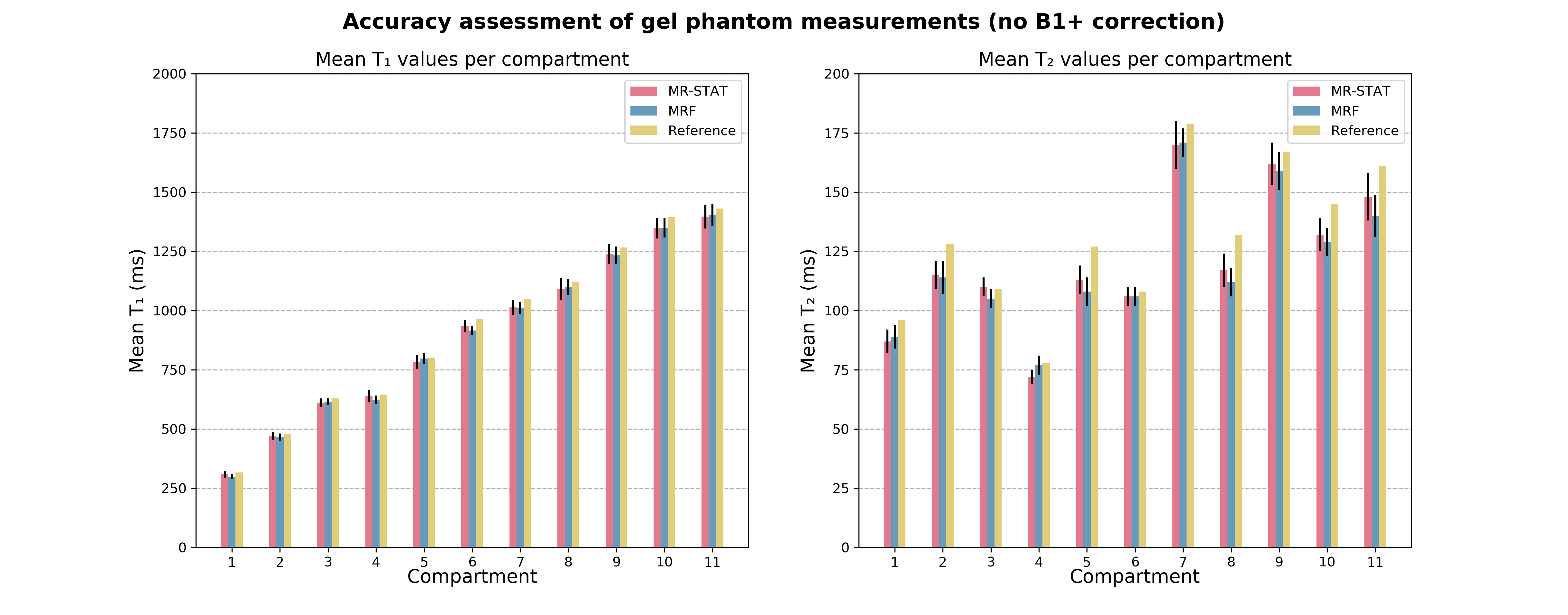
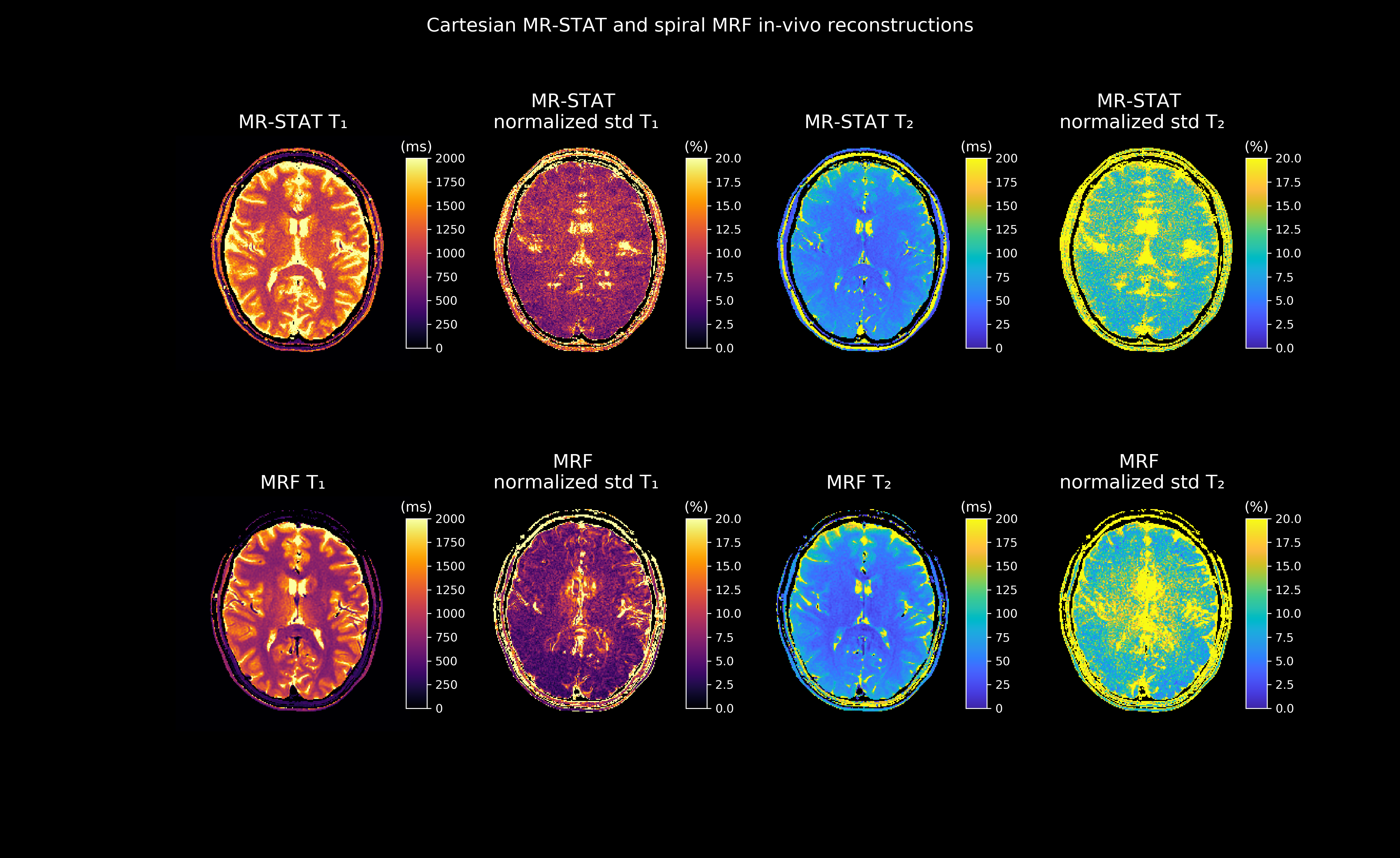
In Fig. 2, first and third columns, the T1 and T2 maps of the gel phantoms obtained using MRF and MR-STAT are shown (first of the ten repetitions). From Fig. 3 it can be observed that both methods demonstrate excellent agreement with gold standard measurements. In Fig. 2, second and fourth columns, voxel-wise standard deviations over T1 and T2 maps of the ten reconstructions, divided by the voxel-wise means, are displayed. The average normalized standard deviations over all tubes for MR-STAT are 3.4% (T1) and 4.9% (T2) whereas for MRF they are 2.3% (T1) and 3.9% (T2).The in-vivo reconstructions (first of ten repetitions) and standard deviation maps are shown in Fig. 4. The parameter maps from both methods are visually comparable. However, we do observe a significant difference in T1 estimates, especially in white matter.
In Fig. 5, we compute the difference between the first out of ten in-vivo reconstructions and the average of the ten reconstructions. This should give an estimate of noise in the parameter maps. Noise spectra obtained by applying the FFT are displayed. We observe a circularly symmetric decay in spiral MRF noise spectra that likely results from not measuring outer corners of k-space with spiral acquisitions.
Discussion
Both Cartesian MR-STAT and spiral MRF are successful in estimating T1 and T2 values from short 2D scans in gel phantoms as well as in-vivo. With the sampling and reconstruction setup used in the current work, spiral MRF returns parameter maps with higher precision. However, interpretation of the precision estimates are complicated by the fact that spiral MRF does not sample the outer corners of k-space whereas in Cartesian MR-STAT a k-space apodization (Riesz filter) is applied prior to reconstruction. Both techniques suppress high spatial frequencies and therefore noise differently (see Fig. 5). For an in-depth analysis one would have to compensate for these mechanisms.The larger difference between the two acquisitions resides in the in-vivo maps. Because both sequences have different RF power depositions (different time-varying flip angle trains, slice-selective vs non-selective inversion) the observed differences in T1 estimates between MR-STAT and MRF may be due to magnetization transfer effects.6,7,8
In the current work, no B1-transmit field correction has been applied. Correcting for the B1-transmit bias may improve the accuracy of T2 estimates.9
Conclusion
Spiral MRF and Cartesian MR-STAT both result in high quality T1 and T2 parameter maps. A thorough performance analysis is subject to choice of acquisition/reconstruction parameters and therefore not straightforward. The clinical application at hand may dictate a preference of one method over the other.Acknowledgements
This research has been financed by the Dutch Technology Foundation under grant #17986.References
[1] Ma, D et al. Magnetic Resonance Fingerprinting. Nature 495 (2013): 187–192.
[2] Sbrizzi, A et al. Fast quantitative MRI as a nonlinear tomography problem. Magnetic Resonance Imaging 46 (2018): 56-63.
[3] Fuderer, M et al. Efficient performance analysis and optimization of transient-state sequences for multi-parametric MRI. NMR in Biomedicine. doi: 10.1002/nbm.4864.
[4] van der Heide, O et al. High‐resolution in vivo MR‐STAT using a matrix‐free and parallelized reconstruction algorithm. NMR in Biomedicine 33.4 (2020): e4251.
[5] McGivney, DF et al. SVD compression for magnetic resonance fingerprinting in the time domain. IEEE Trans Med Imaging. 2014 Dec; 33(12):2311-22.
[6] van Gelderen P, et al. Effects of magnetization transfer on T1 contrast in human brain white matter. Neuroimage. 2016 Mar;128:85-95.
[7] Teixeira AG et al. Controlled saturation magnetization transfer for reproducible multivendor variable flip angle T1 and T2 mapping. Magn Reson Med. 2020 Jul; 84(1):221-236.
[8] Hilbert T, et al. Magnetization transfer in magnetic resonance fingerprinting. Magn Reson Med. 2020 Jul; 84(1):128-141.
[9] Buonincontri G, et al. MR fingerprinting with simultaneous B1 estimation. Magn Reson Med. 2016; 76:1127–1135.
Figures