2186
Iterative denoising of undersampled 3D MRF with exact line search and spatial regularization1NMR Laboratory, Neuromuscular Investigation Center, Institute of Myology, Paris, France
Synopsis
Keywords: MR Fingerprinting/Synthetic MR, Sparse & Low-Rank Models
We propose an iterative algorithm to remove remaining artefacts of Magnetic Resonance Fingerprinting maps, using projected gradient descent with exact line search and spatial regularization. We use this framework to denoise 3D MRF T1-FF acquisitions undersampled in the partition direction and show that this allows to reduce undersampling artefacts for the T1H2O and FF maps after a few iterations.Introduction
Fat fraction (FF) and water T1 (T1H2O) could have great potential in assessing neuromuscular disorders severity and activity [1]. FF and T1H2O can be jointly estimated in an efficient way using MR Fingerprinting (MRF) [2,3]. Although MRF reconstruction through dictionary matching removes most undersampling artefacts due to their incoherence along timesteps, some might remain, especially at high acceleration factors. Compressed Sensing (CS) frameworks for MRF [4] have been proposed to denoise the parameter maps, however an explicit solution for the optimal gradient step is missing. We introduce an iterative denoising framework using exact line search and spatial regularization, and demonstrate its performance on 3D MRF T1-FF data undersampled in the partition direction [5].Theory
The 3D MRF problem consists in building time-series of 3D volumes while matching the temporal evolution of each pixel to a precomputed dictionary. This can be seen as the least square reconstruction of temporal volumes under the low-rank constraint for each pixel evolution to be described by one element of the dictionary. We added Total Variation regularization (TV) in the three spatial directions in order to improve the convergence:$$argmin_{X \in D}J(X)+\lambda||TV(X)||_1\\J(X)=‖𝑊^{\frac{1}{2}}(𝐴𝑋−𝑌)‖_2^2$$
Where X represents the time series of image to be reconstructed (shape NxT where N is total number of pixels and T is the number of temporal steps), Y represents the acquired k-space data (NcPxT where Nc is the number of coils and P is the number of k-space samples for each timestep), A=FΩC is the multi coil Fourier transform, where F is the Fourier operator, Ω is the undersampling operator and C are the coil sensitivities (NcPxN), D is the dictionary of precomputed fingerprints, and W are weights that allow us to precondition the reconstruction, and accelerate the convergence [6]. More specifically, in our case of radial cylindrical sampling, they correspond to the radial density correction along each spoke (NcPxNcP).
This can be solved iteratively by projected gradient descent [4]. Each iteration consists in the projection of the signals on their best fit $$$ \widehat{X}$$$ in the dictionary through a pattern matching algorithm [6], together with a gradient descent update on the cost function for data consistency:
$$\widehat{X}\leftarrow\widehat{X}+\mu\nabla J(\widehat{X})+\lambda\nabla||TV(\widehat{X})||_1\\\nabla J(\widehat{X})=2U(AX-Y)$$
Where $$$U=A^HW$$$ is the inverse Fourier transform with density compensation.
We propose here to use the closed form formula given by the exact line search for choosing the optimal $$$\mu$$$ ($$$\mu_{opt}$$$). In most cases, doing exact line search is intractable due to gradient calculation, however in our specific case this can be calculated in a straightforward way (Figure 2):
$$\mu_{opt}=-0.5\frac{||\nabla J(\widehat{X})||_2^2}{<WA\nabla J(\widehat{X}),A\nabla J(\widehat{X})>}$$
The only additional calculation required at each step to get $$$\mu_{opt}$$$ is hence the Fourier Transform of the already calculated gradient ($$$ A\nabla J(\widehat{X})$$$).
Methods
We validated this methodology on a 3D MRF T1-FF sequence, which consists of a stack of golden angle radial acquisitions. The partition direction was further undersampled by 4 as described in [5].We tested on both numerical phantoms (resolution 16x64x64, 64 squared subregions of size 4x4 in each of the 16 slices with uniform FF, T1H2O, B1 and Df values) and in vivo on 3D undersampled axial acquisitions on the thighs of one healthy volunteer (34 coils, 80 slices , resolution 5x1x1mm3, FOV 40x29.3x29.3cm3) acquired at 3T (PrismaFit, Siemens Healthineers).
On numerical phantoms, the regions of interest (ROIs) correspond to the squared subregions. The accuracy and precision of the proposed algorithm was assessed by calculating the mean and standard deviation of FF and T1H2O estimation errors on all ROIs against the ground truth across iterations of the algorithm.
In vivo, 11 ROIs were drawn manually on right thigh muscles. The precision of the proposed algorithm was evaluated by deriving the mean value of FF and T1H2O and corresponding standard deviation in different regions of interest (ROIs) for each iteration of the algorithm.
Results
Figure 2 shows the cost $$$J(\widehat{X}+ \mu∗\nabla𝐽(\widehat{𝑋̂}))$$$ as a function of $$$\mu$$$ for the first iteration of the reconstruction of the numerical phantom. The theoretical calculation of $$$\mu_{opt}$$$ corresponds well to the minimum of the function, ensuring that J decreases at each timestep.On numerical phantoms, data undersampled 4 times in the partition direction provided the same level of accuracy and better precision than fully sampled data with the standard dictionary matching reconstruction approach in only 3 iterations of the algorithm (Figure 3). The algorithm converged in around 10 iterations, with precision further improved compared to fully sampled data (standard deviation on all ROIs decreased by 2% for FF and 30ms for T1H2O).
On in vivo data, 6 iterations of the algorithm removed the main artefacts introduced by the undersampling in the partition direction (Figure 4). The methodology introduced no significant bias (Figure 5), with a precision comparable to fully sampled data in the partition direction after 3 iterations, and even better precision after 6 iterations (standard deviation on ROIs decreased between 10ms and 30ms for T1H2O).
Discussion & Conclusion
We proposed in this work an iterative method to denoise highly undersampled data from 3D MRF experiments. The method improves the parameter maps after a few iterations.This would allow us to shorten scan time while keeping similar maps precision and accuracy.
Acknowledgements
This study was funded by ANR-20-CE19-0004.References
[1] Marty, B., Reyngoudt, H., Boisserie, J. M., le Louër, J., Araujo, E. C. A., Fromes, Y., & Carlier, P. G. (2021). Water-fat separation in mr fingerprinting for quantitative monitoring of the skeletal muscle in neuromuscular disorders. Radiology, 300(3), 652–660. https://doi.org/10.1148/radiol.2021204028
[2] Ma, D., Gulani, V., Seiberlich, N., Liu, K., Sunshine, J. L., Duerk, J. L., & Griswold, M. A. (2013). Magnetic resonance fingerprinting. Nature, 495(7440), 187–192. https://doi.org/10.1038/nature11971
[3] Marty, B., & Carlier, P. G. (2020). MR fingerprinting for water T1 and fat fraction quantification in fat infiltrated skeletal muscles. Magnetic Resonance in Medicine, 83(2), 621–634. https://doi.org/10.1002/mrm.27960
[4] Davies, M., Puy, G., Vandergheynst, P., & Wiaux, Y. (2014). A compressed sensing framework for magnetic resonance fingerprinting. SIAM Journal on Imaging Sciences, 7(4), 2623–2656. https://doi.org/10.1137/130947246
[5] Marty, B., Lopez Kolkovsky, A. L., Araujo, E. C. A., & Reyngoudt, H. (2021). Quantitative Skeletal Muscle Imaging Using 3D MR Fingerprinting With Water and Fat Separation. Journal of Magnetic Resonance Imaging, 53(5), 1529–1538. https://doi.org/10.1002/jmri.27381
[6] Johnson, K. M., Block, W. F., Reeder, S. B., & Samsonov, A. (n.d.). Improved Least Squares MR Image Reconstruction Using Estimates of k-Space Data Consistency. https://doi.org/10.1002/mrm.23144
[7] Slioussarenko, C., Baudin ,P.Y. , Reyngoudt, H. & Marty, B (2022). Bi-component dictionary for efficient quantification of fat fraction and water T1 via MR fingerprinting. ISMRM Proc 2022
Figures
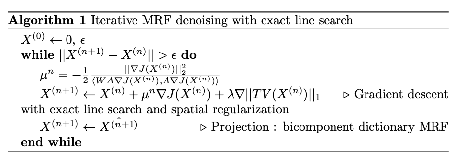
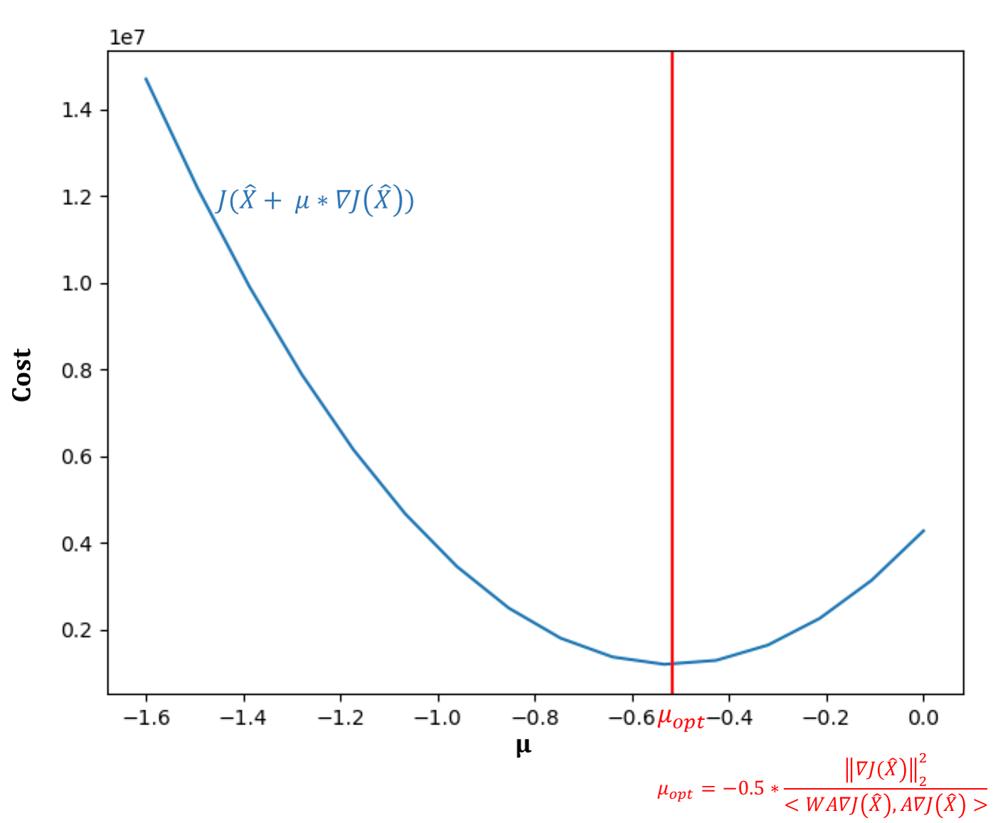
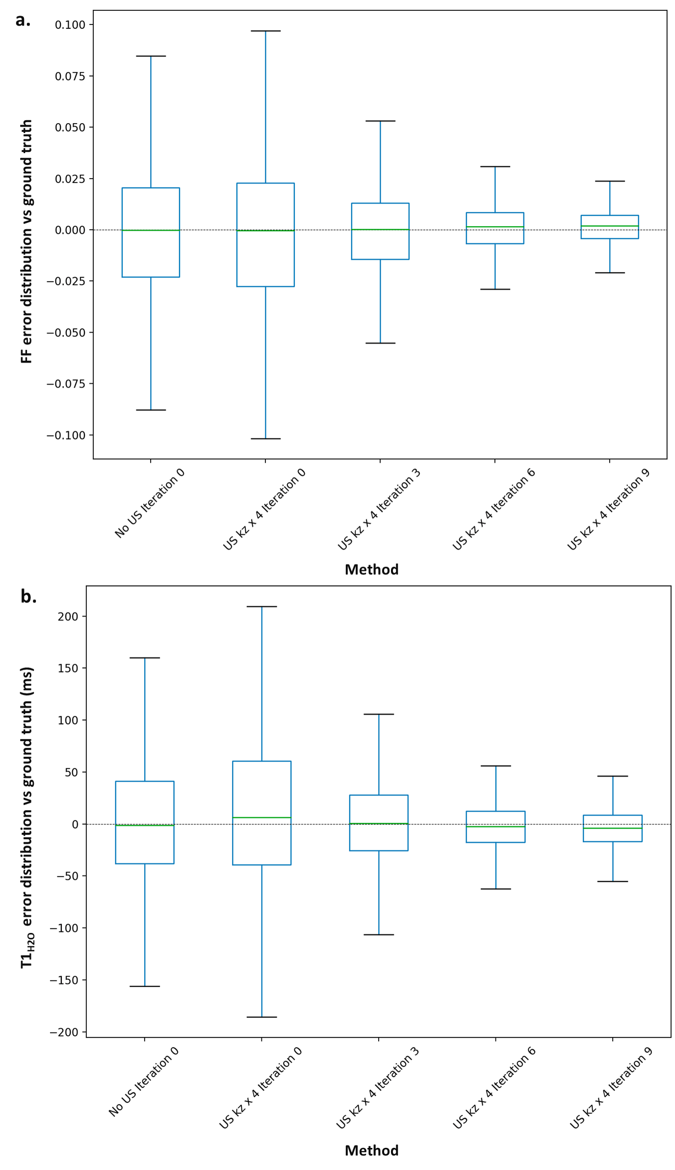
Fig 3. : Numerical phantom parameter estimation error against ground truth for fully sampled MRF data (No US) and for 4 x undersampled (4xUS) MRF data in the partition direction for iterations
0,3,6,9 ot the denoising algorithm
a. Box plot of FF estimation error against ground truth on all ROIs
b. Box plot of T1H2O estimation error against ground truth on all ROIs
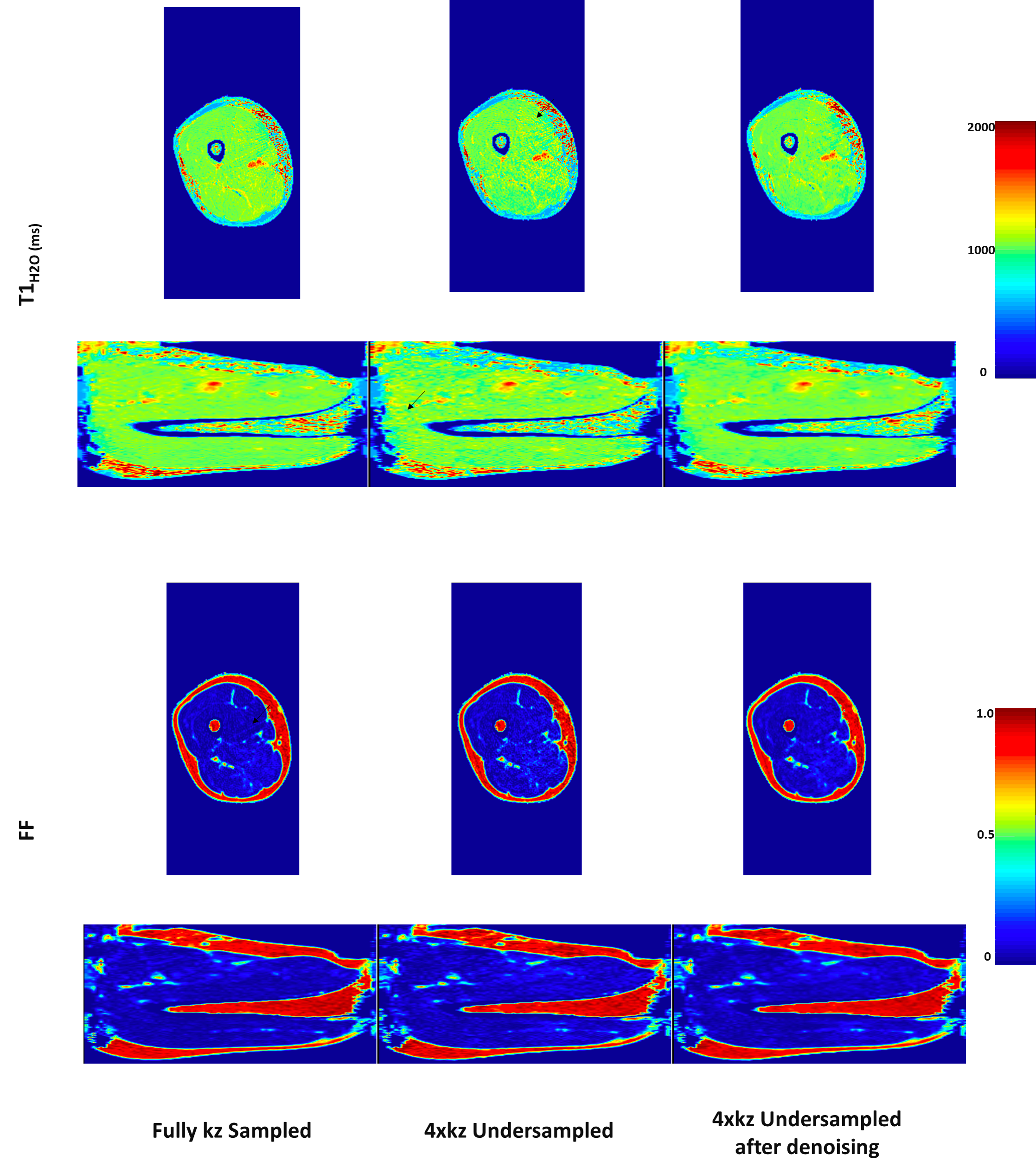
Fig 4: T1H2O and FF maps in one slice (axial view first row, coronal view second row) of the right thigh of one healthy volunteer. From left to right : fully sampled in the partition direction after simple dictionary matching, 4 x undersampled in the partition direction after simple dictionary matching, 4 x undersampled in the partition direction after 6 iterations of the denoisnig algorithm.
One can see that the iterative denoising algorithm removes artefacts introduced by the undersampling (black arrows).
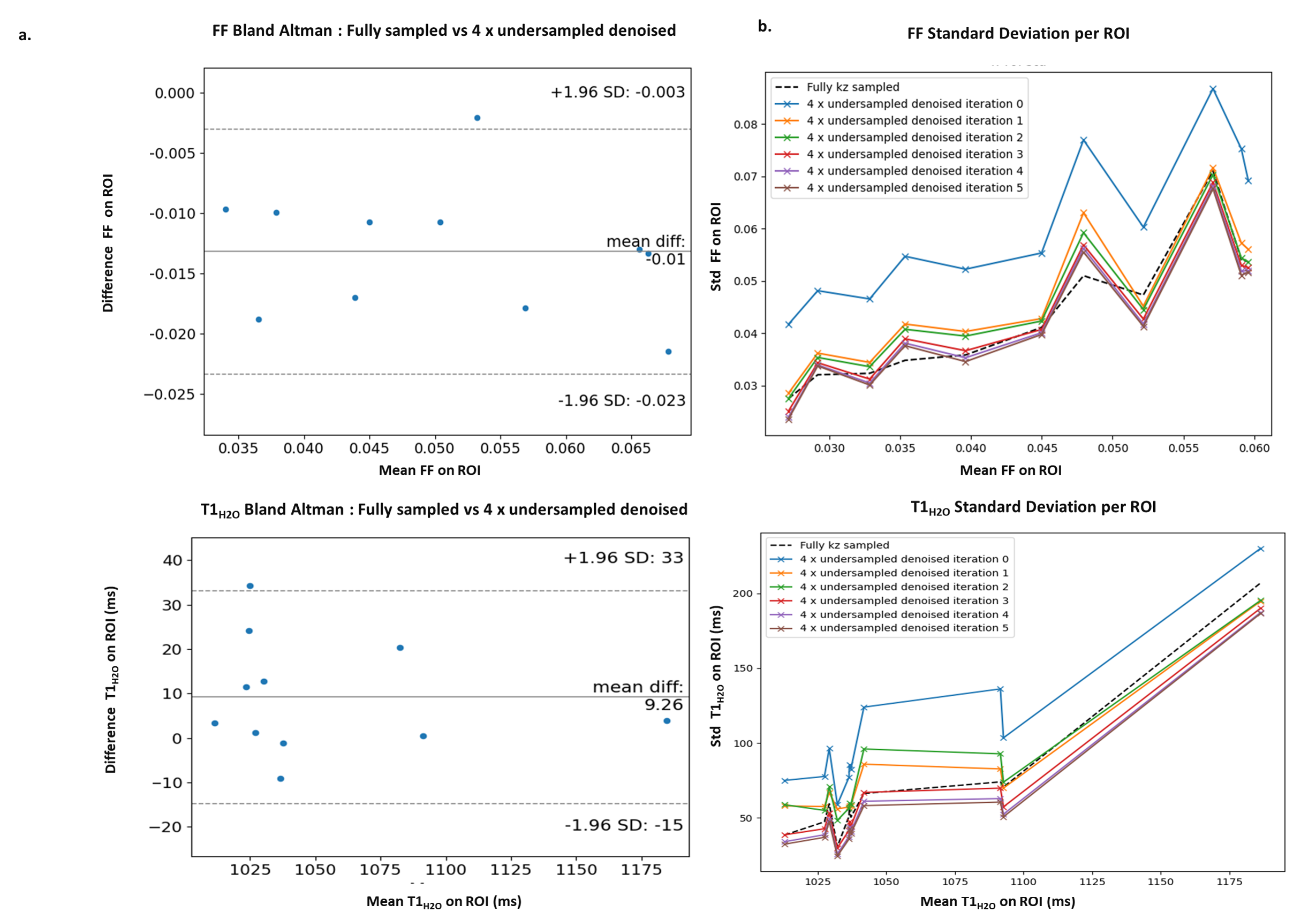
Fig. 5: In vivo comparison of fully sampled in the partition direction against 4 x undersampled after applying denoising algorithm, on the 11 ROIs drawn in the right thigh muscles of one healthy volunteer
a. Bland Altman plots for T1H2O and FF in each ROIs of fully sampled against 4 x undersampled in the partition direction after 6 iterations of the denoising algorithm
b. Standard deviation of T1H2O and FF estimation in each ROIs for the 6 first iterations of the denoising algorithm.